BJT DC analysis

BJT DC analysis is the procedure for finding a BJT’s operating point — the DC values $I_C$, $I_B$, $I_E$, $V_{CE}$ — with no signal applied. You almost always assume active mode, solve, then check the assumption; if it fails the device is in saturation and you redo it.

The recipe

1. Assume active mode. This lets you use $V_{BE}=0.7\text{V}$ and $I_C=\beta I_B$ (the BJT large-signal model).
2. Set $V_{BE}=0.7\text{V}$ (constant-voltage-drop EBJ).
3. KVL around the input (base–emitter) loop to find $I_B$ — or, for a divider bias, find the base voltage $V_B$ from the divider.
4. Compute the currents: $I_C=\beta I_B$ and $I_E=(\beta +1)I_B$. (Equivalently $I_C=\alpha I_E$, with $\alpha \approx 1$.)
5. KVL around the output (collector–emitter) loop to find $V_{CE}$.
6. Check the assumption. If $V_{CE}>0.3\text{V}$ (npn), the CBJ really is reverse-biased — active mode confirmed, the answer stands. If $V_{CE}<0.3\text{V}$ (or comes out negative), active mode is impossible: the device is in saturation. Redo with $V_{CE}=V_{CE(\text{sat})}=0.2\text{V}$ as known and let $I_C$ fall out of the external circuit; $\beta I_B$ no longer holds.

Four-resistor (voltage-divider) topology

The standard discrete bias. $R_{B1}$ and $R_{B2}$ form a divider from $V_{CC}$ to ground setting the base voltage $V_B$; $R_C$ runs collector to $V_{CC}$; $R_E$ runs emitter to ground. The fast path:

• $V_B$ from the divider (assuming the divider current ≫ $I_B$ so base loading is negligible).
• $V_E=V_B-V_{BE}$.
• $I_E=V_E/R_E$.
• $I_C\approx I_E$ (since $\alpha \approx 1$).
• $V_C=V_{CC}-I_C{R}_C$.
• Check $V_{CE}=V_C-V_E>0.3\text{V}$ to confirm active mode.

This is robust against $\beta$ variation precisely because the bias current is set by resistors ($V_E/R_E$), not by $\beta$. See Voltage-divider bias and Discrete-circuit BJT amplifier.

$V_{CC}=10\text{V}$, base driven directly at $V_{BB}=4\text{V}$, $R_C=4.7\text{k}\Omega$, $R_E=3.3\text{k}\Omega$, $\beta =100$. Active gives $V_E=3.3\text{V}$, $I_E\approx 1\text{mA}$, $V_C=5.3\text{V}$ — active confirmed.

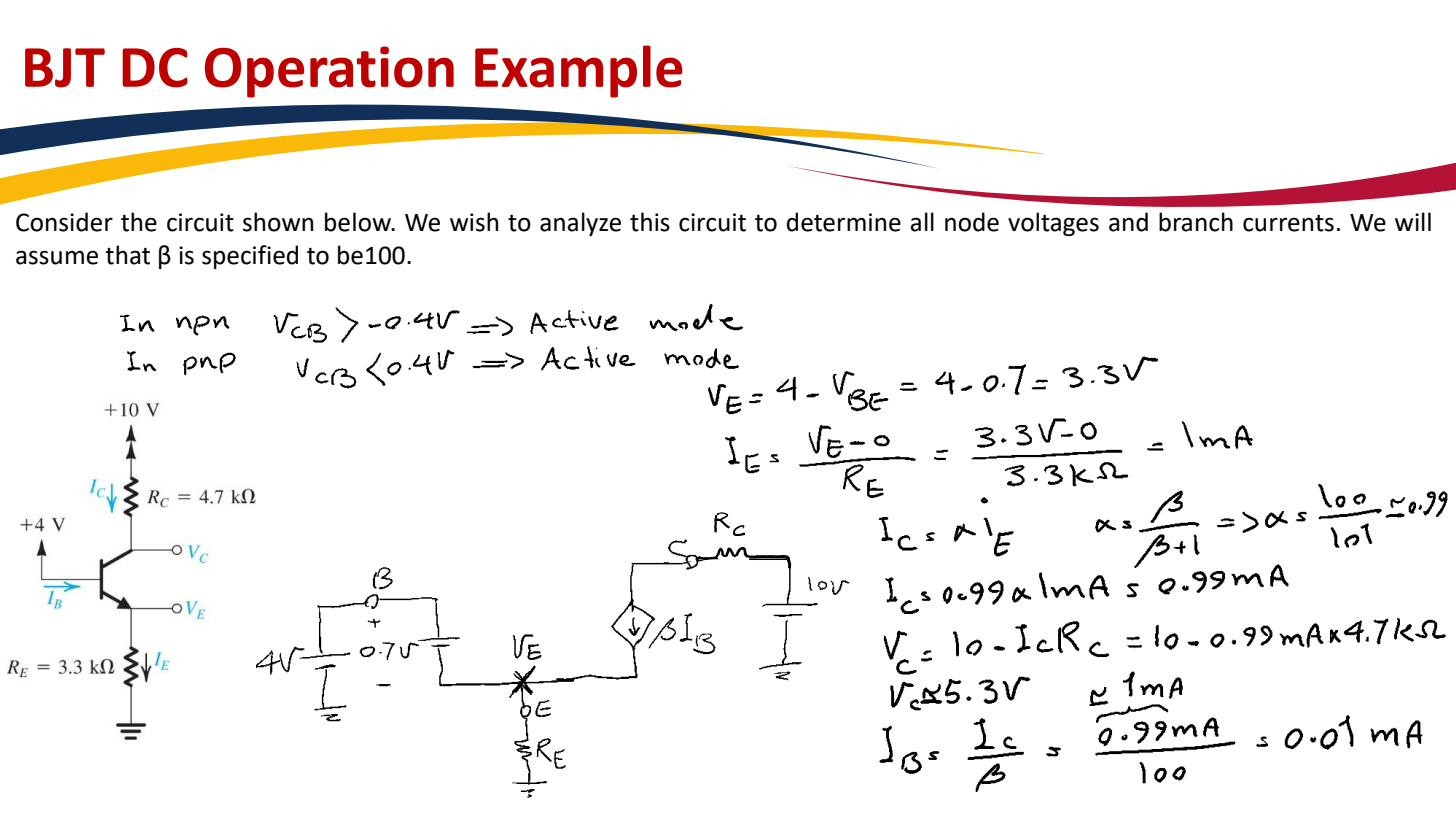
Worked example 1 — active mode confirmed

$V_{CC}=10\text{V}$; the base is driven directly from a $V_{BB}=4\text{V}$ source; $R_C=4.7\text{k}\Omega$ from collector to $V_{CC}$; $R_E=3.3\text{k}\Omega$ from emitter to ground; $\beta =100$.

• Assume active, $V_{BE}=0.7\text{V}$. Emitter voltage: $V_E=V_{BB}-V_{BE}=4-0.7=3.3\text{V}$.
• Emitter current: $I_E=V_E/R_E=3.3/3.3\text{k}=1\text{mA}$.
• $I_C=\alpha I_E=\frac{\beta }{\beta +1}{I}_E=\frac{100}{101}(1\text{mA})\approx 0.99\text{mA}$; base current $I_B=I_C/\beta \approx 9.9\mu \text{A}$.
• Collector voltage: $V_C=V_{CC}-I_C{R}_C=10-(0.99\text{mA})(4.7\text{k})\approx 5.3\text{V}$.
• Check: $V_{CE}=V_C-V_E=5.3-3.3=2.0\text{V}>0.3\text{V}$ (equivalently $V_{CB}>-0.4\text{V}$). Active mode confirmed; the operating point is valid.

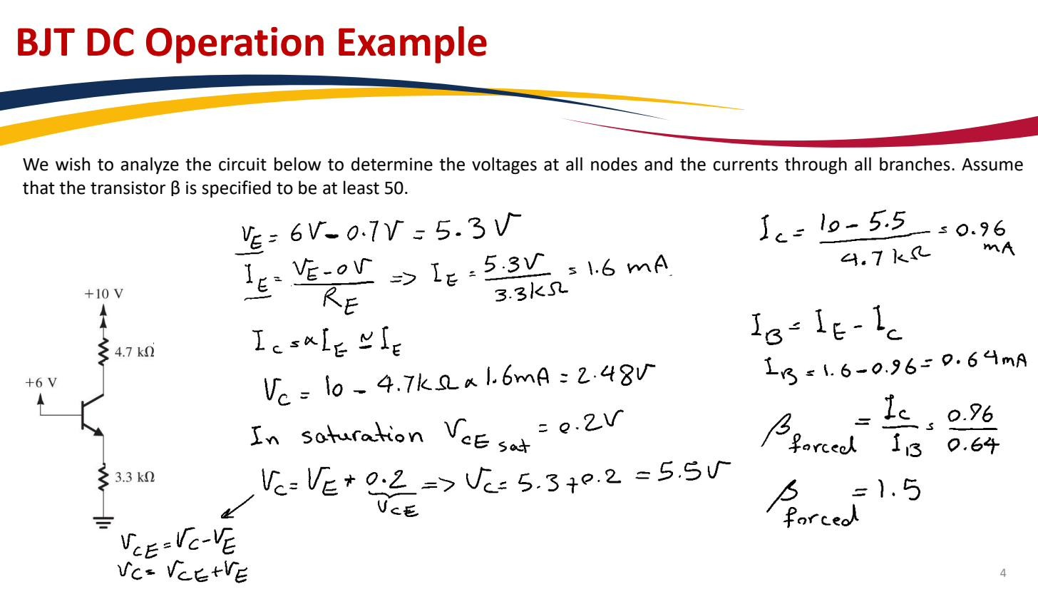
Worked example 2 — active assumption FAILS (saturation)

Same circuit but the base source is now $V_{BB}=6\text{V}$ ($V_{CC}=10\text{V}$, $R_C=4.7\text{k}\Omega$, $R_E=3.3\text{k}\Omega$, $\beta \ge 50$).

• Assume active: $V_E=6-0.7=5.3\text{V}$, so $I_E=5.3/3.3\text{k}\approx 1.6\text{mA}$, $I_C\approx 1.6\text{mA}$.
• Predicted $V_C=10-(4.7\text{k})(1.6\text{mA})=10-7.52=2.48\text{V}$.
• Check fails: $V_C=2.48\text{V}$ is below $V_E=5.3\text{V}$, so $V_{CE}<0$ — impossible. The active assumption is wrong; the device is in saturation.
• Redo in saturation: use $V_{CE}=V_{CE(\text{sat})}=0.2\text{V}$. The base is still pinned at $V_{BB}=6\text{V}$ with $V_{BE}\approx 0.7\text{V}$, so $V_E$ stays at $V_{BB}-V_{BE}=5.3\text{V}$ and $I_E=V_E/R_E=5.3/3.3\text{k}\approx 1.6\text{mA}$. From $V_{CE(\text{sat})}$: $V_C=V_E+0.2=5.5\text{V}$, so $I_C=(V_{CC}-V_C)/R_C=(10-5.5)/4.7\text{k}\approx 0.96\text{mA}$, set entirely by the external collector loop (not by $\beta I_B$). The base current then falls out of KCL: $I_B=I_E-I_C\approx 1.6-0.96\approx 0.64\text{mA}$. Hence ${\beta }_{\text{forced}}=I_C/I_B\approx 0.96/0.64\approx 1.5$ — far below the device $\beta \ge 50$, the tell-tale signature of hard saturation. The whole point of this workflow: in saturation the base is being driven harder than the collector circuit can absorb, so $I_C$ saturates at the external limit and the excess base drive shows up as ${\beta }_{\text{forced}}\ll \beta$. This is the standard “assume active, then check” loop.

The $V_{BB}=6\text{V}$ case predicts $V_{CE}<0$ — the active assumption fails; redo with $V_{CE(\text{sat})}=0.2\text{V}$, giving ${\beta }_{\text{forced}}\approx 1.5$.

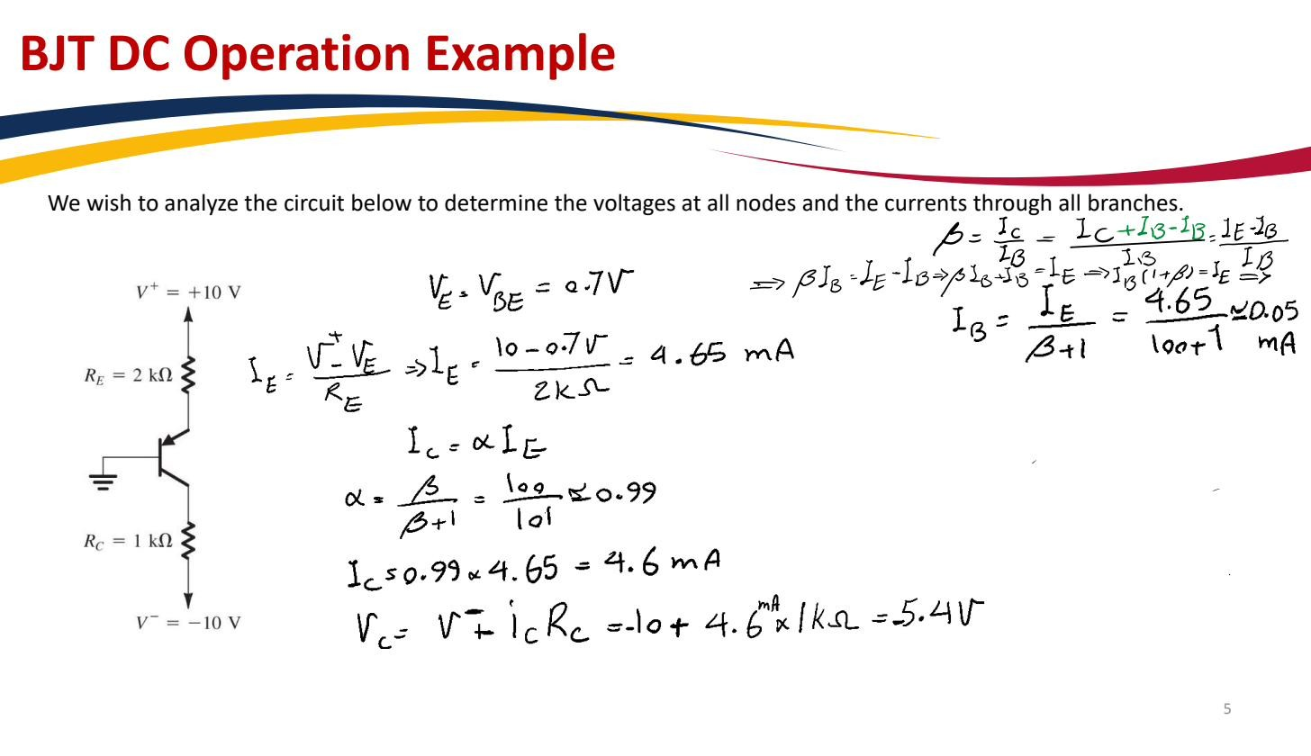
Worked example 3 — pnp on dual supplies

A pnp biased between $+10\text{V}$ and $-10\text{V}$; $R_E=2\text{k}\Omega$ from the emitter to the $+10\text{V}$ rail; $R_C=1\text{k}\Omega$ from the collector to the $-10\text{V}$ rail; base referenced to ground; $\beta =100$.

For a pnp the EBJ is forward-biased with the emitter positive relative to the base, so $V_{EB}=0.7\text{V}$. With the base at ground, the emitter sits at $V_E=+0.7\text{V}$.

• Emitter current (out of the $+10\text{V}$ rail through $R_E$): $I_E=\frac{V^{+}-V_E}{R_E}=\frac{10-0.7}{2\text{k}}=\frac{9.3}{2\text{k}}=4.65\text{mA}$.
• $I_C\approx \alpha I_E\approx 4.6\text{mA}$ (flowing out of the collector for a pnp).
• Collector voltage: $V_C=V^{-}+I_C{R}_C=-10+(4.6\text{mA})(1\text{k})=-10+4.6=-5.4\text{V}$.
• Check: for a pnp, active mode needs the CBJ reverse-biased — here $V_C=-5.4\text{V}$ is well below $V_E=+0.7\text{V}$, so $V_{EC}=0.7-(-5.4)=6.1\text{V}\gg 0.2\text{V}$. Active mode verified.

pnp on ±10 V, $R_E=2\text{k}\Omega$, $R_C=1\text{k}\Omega$, $\beta =100$: $V_E=0.7\text{V}$, $I_E=4.65\text{mA}$, $I_C\approx 4.6\text{mA}$, $V_C=-5.4\text{V}$ — active verified.

The whole point of robust topologies (Voltage-divider bias, dual-supply, Emitter degeneration) is to make the operating point depend on resistor ratios and supply voltages, not on the poorly-controlled $\beta$.