BJT large-signal model

The BJT large-signal model is the DC equivalent circuit you substitute for a BJT when finding its operating point. In active mode it has two pieces: the emitter–base junction modelled as a forward-biased diode, and the collector modelled as a current source controlled by the base current.

The active-mode model

• Emitter–base junction: a forward diode. For hand analysis use the Constant-voltage-drop model — replace it by a fixed $V_{BE}\approx 0.7\text{V}$ from base to emitter.
• Collector: a current source equal to $\beta$ times the base current, pointing into the collector for an npn:

$i_C=\beta i_B=I_S{e}^{V_{BE}/V_T}$

where $\beta$ is the Common-emitter current gain, $I_S$ the saturation current, and $V_T\approx 25\text{mV}$ the Thermal voltage. The two forms of $i_C$ are the same physical current expressed two ways.

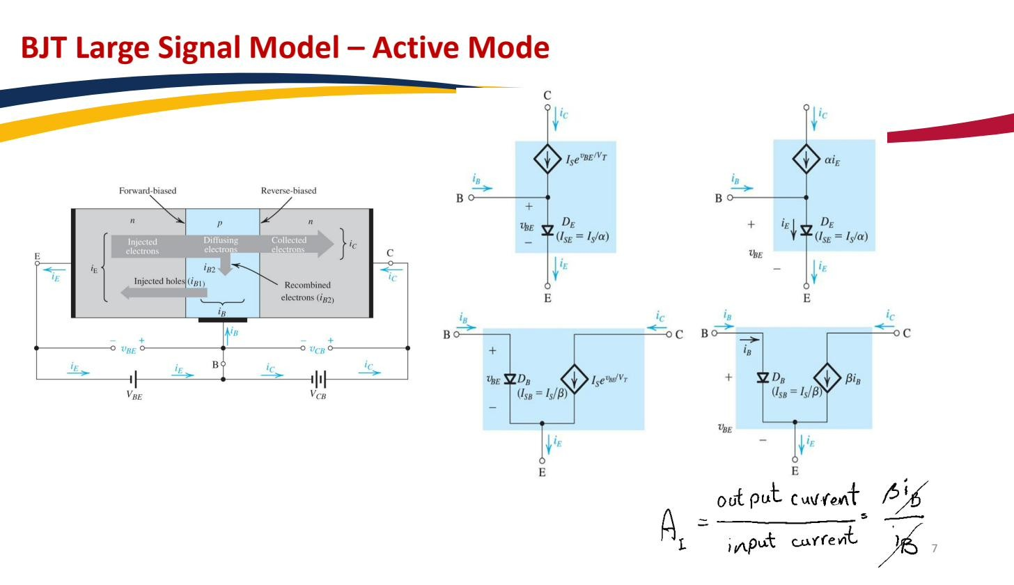BJT large-signal model in active mode: the EBJ is a diode with $V_{BE}\approx 0.7\text{V}$; the collector is a current source $i_C=\beta i_B=I_S{e}^{V_{BE}/V_T}$.

CVD-mode versus exponential-mode

There are two equivalent ways to use this model, and they give nearly the same numbers:

• CVD mode (constant-voltage-drop): fix $V_{BE}=0.7\text{V}$. Then $I_C$ is whatever the external circuit forces through $I_C=\beta I_B$. This is the standard recipe in BJT DC analysis — almost always good enough.
• Exponential mode: keep the full law $I_C=I_S{e}^{V_{BE}/V_T}$, so $V_{BE}$ and $I_C$ are linked and both adjust to the external circuit. More accurate, more algebra.

They agree closely because the exponential is so steep that $V_{BE}$ moves only a few tens of millivolts across orders of magnitude of $I_C$ — so pinning it at 0.7 V costs almost nothing. Use CVD mode unless a problem specifically demands the exponential.

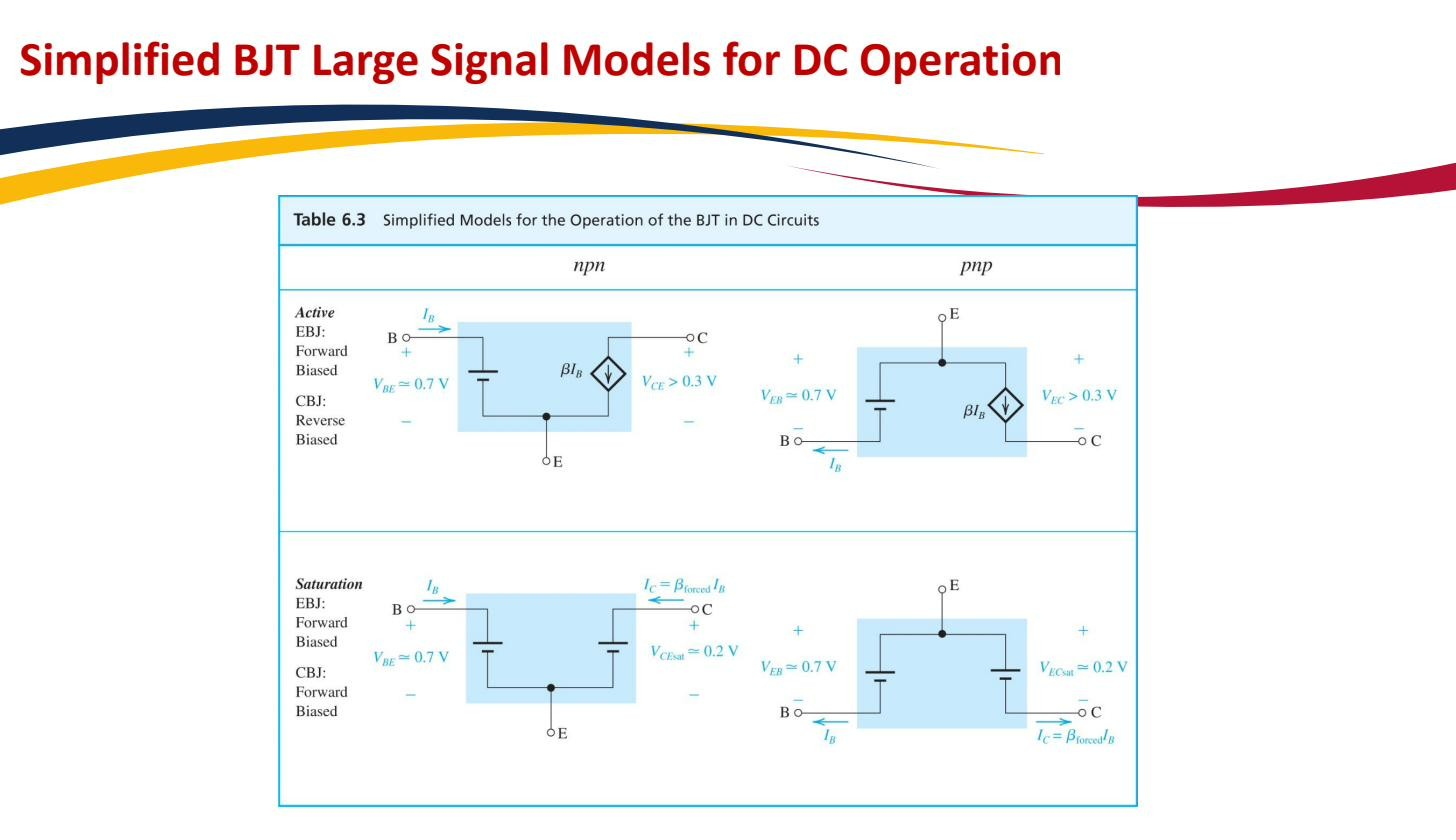
Simplified model: drop the Early effect

The full active-mode model also includes an output resistance $r_o$ from the Early effect (collector current rising slightly with $v_{CE}$). For introductory DC hand analysis you drop $r_o$ (treat the collector as an ideal current source), which gives the standard ”$V_{BE}=0.7\text{V}$, $I_C=\beta I_B$” model used in nearly every textbook bias problem.

Drop the Early effect for hand analysis at this level — that gives the standard ”$V_{BE}=0.7\text{V}$, $I_C=\beta I_B$” model used in most introductory problems.

A separate large-signal model applies in saturation (fixed $V_{BE}\approx 0.7\text{V}$ and fixed $V_{CE(\text{sat})}\approx 0.2\text{V}$), and the pnp version has the diode and current-source directions reversed. Once the DC operating point is known, you linearise this model around it to get the BJT small-signal model.