The confusion matrix is a 2×2 table (for binary classification) that records every possible combination of true class and predicted class. It’s the starting point for evaluating a classifier: every other binary classification metric is derived from these four counts.
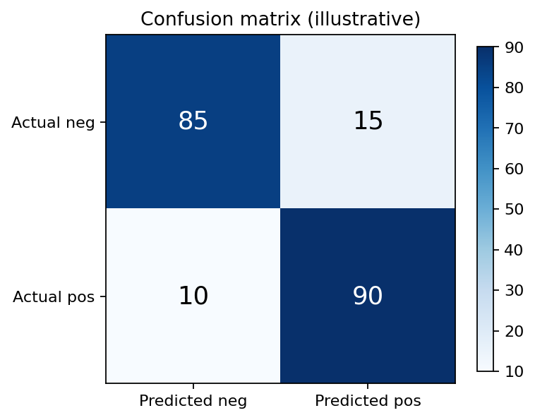 Example 2x2 confusion matrix with rows = actual class and columns = predicted class.
For a binary classification problem with class 1 designated as the positive class and class 0 as the negative class, four outcomes are possible for any single test example:
- True positive (TP): actually positive, predicted positive. Good prediction.
- True negative (TN): actually negative, predicted negative. Also good.
- False positive (FP) — actually negative, predicted positive. Sometimes called a Type I error.
- False negative (FN) — actually positive, predicted negative. Type II error.
The confusion matrix arranges these four counts into a 2×2 table. There are conventions in both directions — some put predicted on rows and actual on columns, some the reverse. scikit-learn (and the example below) puts true classes on the rows and predicted classes on the columns, with confusion_matrix(y_true, y_pred) returning . Always check the axis labels before reading a confusion matrix — getting the orientation wrong swaps FP with FN.
The two diagonals tell two different stories. The main diagonal (TP and TN) is where the model gets things right. The off-diagonal (FP and FN) is where it makes mistakes. A perfect classifier has all counts on the main diagonal and zeros off it.
Realistic classifiers have nonzero entries in all four cells. A good way to visualize them is as a Heat map: brighter colors on cells with more examples, dimmer on cells with fewer. A classifier working well shows a bright main diagonal and a dim off-diagonal.
Metrics from the confusion matrix
From the four numbers we can compute several scalar metrics, each capturing a different aspect of performance:
- Accuracy: fraction of predictions that are correct.
- Recall (sensitivity, TPR): of actual positives, how many did the classifier catch?
- Specificity (TNR): of actual negatives, how many did the classifier correctly identify?
- Precision: of predicted positives, how many were actually positive?
- F1 score: harmonic mean of precision and recall.
- False positive rate (FPR): of actual negatives, how many were wrongly flagged?
For binary classification, these six are the standard summary. Multi-class classification has a larger confusion matrix (one row and column per class) and analogous per-class metrics.
In scikit-learn
from sklearn.metrics import confusion_matrix, ConfusionMatrixDisplay
cm = confusion_matrix(y_test, y_pred)
ConfusionMatrixDisplay(cm).plot()
A typical output for the wine-quality classifier from the Introduction to Data Science textbook:
              Predicted 0   Predicted 1
True 0:           405           330
True 1:           194          1021
Reading: 405 TN (low-quality, correctly classified), 1021 TP (high-quality, correctly classified), 330 FP (low-quality but called high), 194 FN (high-quality but called low). The classifier is more eager to predict high quality than low quality — recall is 1021/1215 ≈ 0.840, but specificity is only 405/735 ≈ 0.551. That’s a real and informative observation that a single accuracy number wouldn’t reveal.