Slope field

A slope field (or direction field) for a first-order ODE $y^{\prime }=f(x,y)$ is a graphical depiction of the right-hand side: at every point $(x,y)$ in some grid, draw a small line segment with slope $f(x,y)$. The slope field shows the direction a solution would head if it passed through that point, without computing the actual trajectories.

Slope fields make ODEs visual. You can sketch a candidate solution by following the slope arrows from any starting point — the curve threads through the field.

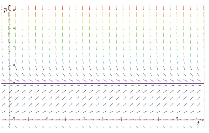
Example: $\frac{dp}{dt}=k(p-2)$

For $\frac{dp}{dt}=k(p-2)$ with $k>0$ (constant), slopes:

• For $p>2$: $k(p-2)>0$, slope positive — solutions grow without bound.
• For $p<2$: slope negative — solutions decrease without bound.
• At $p=2$: slope zero — equilibrium.

The equilibrium at $p=2$ is unstable: trajectories in either neighbourhood are pushed away from it. So calling this “linearized population dynamics” is misleading — real population models (Malthusian, logistic) have stable equilibria around the carrying capacity. This linear model has the equilibrium repelling, not attracting; an actual population starting near $p=2$ would either crash to zero or explode upward, neither of which is the population dynamics intuition. The slope field reveals the (counter-intuitive) instability immediately, without solving.

What slope fields tell you

1. Equilibria — points where slope is zero. Solutions through these points are constant.
2. Direction of motion at every point.
3. Qualitative behavior of solutions: which equilibria attract trajectories, which repel them.
4. Approximate solution shapes — sketch curves that follow the local slope.

Connection to existence and uniqueness

The Existence and uniqueness theorem uses the slope-field language directly. Continuity of $f(x,y)$ means the slope field has no gaps — you can follow it from any starting point. Continuity of $\partial f/\partial y$ means nearby slopes don’t change too abruptly — solutions can’t merge or branch.

Failure of these conditions shows up visually: a discontinuity in $f$ creates a “hole” in the slope field; a discontinuity in $\partial f/\partial y$ creates regions where multiple slopes overlap.

2D systems: vector fields

For 2D autonomous systems $\{\begin{array}{l}{x}^{\prime }=f(x,y)\\ y^{\prime }=g(x,y)\end{array}$, the natural visualization is a vector field: at each point, draw an arrow pointing in direction $(f,g)$ with magnitude $\sqrt{f^2+g^2}$.

Or, for a slope-style display, just the direction $(f,g)/\sqrt{f^2+g^2}$ — the direction without speed.

This is the higher-dimensional analog of a slope field. Trajectories of the system are curves that follow the vector field — see Phase plane.

Drawing slope fields

By hand:

1. Pick a grid (e.g., $-3\le x,y\le 3$ at integer points).
2. At each grid point, compute $f(x,y)$.
3. Draw a short line segment with that slope.
4. Sketch curves that follow the slopes.

In software (Mathematica, Matlab, Python’s matplotlib): streamplot or quiver functions render slope fields directly.

Limitations

Slope fields are only practical for 1D ODEs ($y^{\prime }=f(x,y)$, drawn in 2D) or 2D autonomous systems (drawn as 2D vector fields in the plane).

Higher dimensions are hard to visualize. For 3D, you can use 3D vector field plots, but they’re cluttered. For 4D and beyond, you usually project onto subspaces or work numerically.

For higher-dimensional analysis, the strategies are: linearize around equilibria (see Locally linear system), use Lyapunov functions (Lyapunov’s method), or simulate numerically.

Related visualizations

• Solution curves (specific trajectories): pick initial conditions, integrate the ODE numerically, plot the result. Each curve threads the slope field.
• Nullclines: curves where one component of the vector field is zero. The $x$-nullcline is where $f=0$ (vertical motion only); the $y$-nullcline where $g=0$ (horizontal motion only). Equilibria are where nullclines intersect.

For phase-plane analysis of 2D systems, see Phase plane and Phase plane behaviour.