Principal Component Analysis

Principal Component Analysis (PCA) is the classic linear approach to Dimensionality reduction. The intuition is easiest to see in two dimensions. Suppose we have a cloud of 2D points and we want to reduce it to 1D. The lazy thing to do is drop the $y$ coordinate — keep only $x$. That works geometrically but loses information: the spread in $y$ is gone entirely. If the cloud has interesting variation in $y$, we’ve thrown it away.

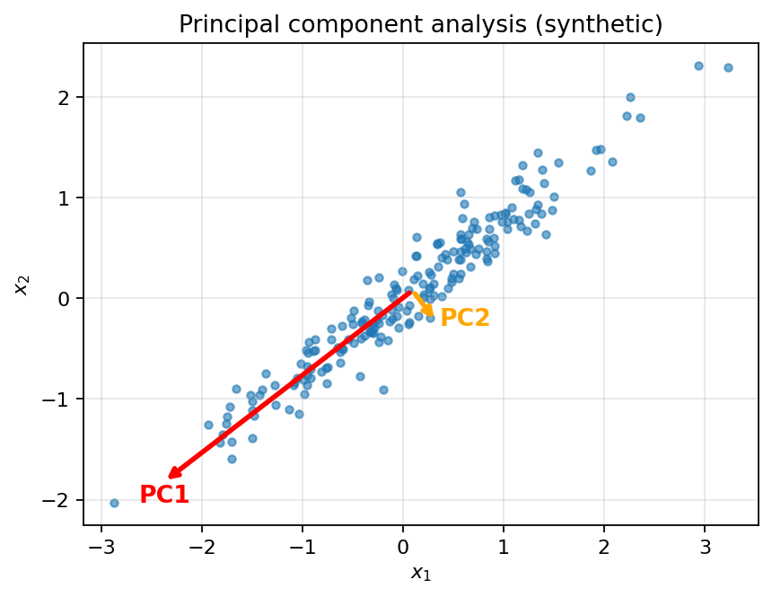
PCA does something smarter. Instead of projecting onto the $x$ or $y$ axis, it asks: is there some other line we could project onto that would preserve more of the variance? Often the answer is yes. If the cloud is elongated along a diagonal, projecting onto that diagonal preserves much more variance than projecting onto either of the original axes.

PCA finds the direction with the highest variance in the data; that’s the first principal component. It then finds the direction with the next-highest variance among directions orthogonal to the first; that’s the second principal component. And so on. Each principal component is a new coordinate axis, and the data, expressed in these new axes, has its variance concentrated in the first few components.

To reduce from $N$ dimensions to $M$, keep the first $M$ principal components and discard the rest. If most of the variance is captured in the first few components — which is often the case in practice — the dropped components contained little variance, and the reduction is nearly lossless with respect to variance. The qualifier matters: PCA preserves variance, not “information” in general. If the meaningful distinction between classes lives along a low-variance direction (a small but important signal masked by a large but uninformative one), PCA will discard exactly the direction we care about. Variance is a useful proxy for information, not the same thing.

Before applying PCA, the data must be centered — every column shifted to have zero mean. Centering is mandatory; without it, the first principal component drifts toward the mean direction rather than the variance direction. When features are on different scales (a column in millimetres versus one in metres), they should also be standardized to unit variance (see Normalization), otherwise the high-magnitude column dominates and PCA gets misled by units rather than structure. StandardScaler in scikit-learn does both centering and standardization.

In Python with scikit-learn:

from sklearn.decomposition import PCA
from sklearn.preprocessing import StandardScaler
 
X = StandardScaler().fit_transform(X)        # normalize
pca = PCA(n_components=2)
X_2d = pca.fit_transform(X)                  # N×2 array

Under the hood

The Introduction to Data Science textbook stops at the conceptual picture and library call. The mathematical machinery — typically left for a later machine-learning course — is worth a quick sketch.

For centered data $X$ ($N$ rows, $D$ features), form the sample covariance matrix $C=\frac{1}{N-1}{X}^{T}X$. This is a $D\times D$ symmetric positive-semidefinite matrix. Its eigenvectors are the principal components: an orthonormal basis of ${\mathbb{R}}^D$ in which $C$ is diagonal. The corresponding eigenvalues ${\lambda }_1\ge {\lambda }_2\ge \cdots \ge {\lambda }_D$ are the variances of the data along those directions. The first principal component (eigenvector with the largest eigenvalue) is the direction of maximum variance — that’s what makes it “principal.”

Equivalently, computed via SVD of the centered data: $X=U\Sigma V^T$. The columns of $V$ are the principal components; the singular values ${\sigma }_i$ relate to the eigenvalues by ${\lambda }_i={\sigma }_i^2/(N-1)$. This is how scikit-learn does it — SVD is numerically more stable than forming $X^{T}X$ explicitly.

The explained variance ratio of component $i$ is ${\lambda }_i/{\sum }_j{\lambda }_j$ — the fraction of total variance captured by that component. Cumulative explained variance after keeping the top $M$ components is ${\sum }_{i=1}^M{\lambda }_i/{\sum }_{j=1}^D{\lambda }_j$. A typical heuristic for choosing $M$ is to pick the smallest $M$ such that the cumulative ratio exceeds 0.9 or 0.95. In scikit-learn this is pca.explained_variance_ratio_.

PCA preserves global linear structure. The complementary technique t-SNE preserves local neighborhood structure and reveals cluster shapes that linear projections can miss. Running both on the same dataset and comparing the plots is informative: PCA tells you the shape of variance, t-SNE tells you the shape of neighborhoods.