A linear autonomous system in the plane is a 2D ODE system of the form
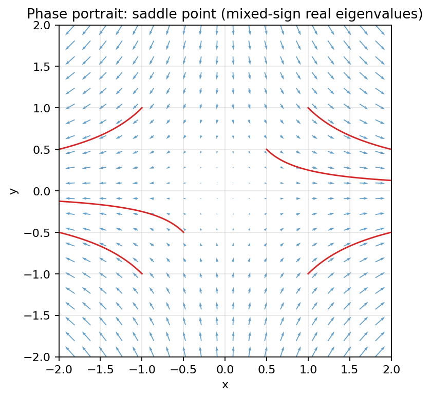 Saddle point: eigenvalues of opposite sign. Trajectories follow the stable manifold in, then peel off along the unstable one.
with constant coefficients . In matrix form:
This is affine in the state, and autonomous in (no on the right).
Reducing to homogeneous
The constants shift the equilibrium away from the origin. By a change of variables, we can move the equilibrium back to the origin and eliminate the constants.
The cleanest way is to shift coordinates to the equilibrium. Solve for the equilibrium (when ), and define . Then
so
Homogeneous, with the equilibrium now at . The new variable is the displacement from equilibrium, geometrically clear.
(An alternative: define new variables to equal the right-hand side, and . The algebra works out to the same homogeneous form, but the geometric meaning is obscured: are velocities of the original system, not coordinate positions, so the phase portrait you draw isn’t directly the original system shifted.)
This change-of-coordinates trick is universal: any linear autonomous system reduces to a homogeneous linear autonomous system after relocating to the equilibrium. So the qualitative analysis (stability, phase portrait) is fully captured by studying .
Eigenvalue classification
For the homogeneous form , the eigenvalues of classify the system’s behavior:
- Distinct real eigenvalues: see Distinct real eigenvalues case.
- Complex conjugate eigenvalues: see Complex conjugate eigenvalues case.
- Repeated eigenvalues: see Repeated eigenvalues case.
The phase portrait (qualitative picture of all trajectories) depends on which case applies. Phase plane behaviour covers the six standard cases.
Why “in the plane”
The 2D case is the most studied because:
- Eigenvalues of a matrix come in pairs that are easy to classify.
- Phase portraits are visualizable as 2D diagrams.
- Most undergraduate ODE courses focus on 2D systems for tractability.
Higher-dimensional linear autonomous systems work the same way (eigenvalues classify behavior), but the geometry gets harder to draw. The 4D case has 4 eigenvalues, with up to two complex pairs, and the phase “portrait” lives in 4D.
Equilibrium location
The equilibrium of satisfies , so when (otherwise there’s no isolated equilibrium).
If , then either there’s no equilibrium (when is not in the column space of ) or there’s a line of equilibria (when is in the column space, multiple work).
For the latter case, you have non-isolated equilibria, and the analysis is different. See Critical point of autonomous system.
In context
The linear autonomous system is the building block for all nonlinear analysis. Near any equilibrium of a nonlinear system, you can linearize (approximate the nonlinear system by its linear part) and the eigenvalue analysis tells you the local behavior. See Locally linear system for this technique.
See Autonomous system and Stability of autonomous systems for the broader picture.