Autonomous system

An autonomous system of ODEs is one whose right-hand side doesn’t depend explicitly on the independent variable $t$:

${\mathbf{x}}^{\prime }=\mathbf{F}(\mathbf{x})$

(no $t$ in $\mathbf{F}$).

The system’s behavior depends only on its current state $\mathbf{x}$, not on what time it is. Same state $\to$ same future evolution, regardless of when you start.

Why autonomous matters

Most physical systems are autonomous when there’s no time-varying external input. The laws of physics don’t care what year it is — only the current configuration of the system matters.

Examples:

• Pendulum (no driving): ${\theta }^{\prime \prime }+(g/L)\sin \theta =0$. Convert to first-order system $(x_1,x_2)=(\theta ,{\theta }^{\prime })$:

$\{\begin{array}{l}{x}_1^{\prime }=x_2\\ x_2^{\prime }=-(g/L)\sin x_1\end{array}$

No $t$ on the right — autonomous.

• Harmonic oscillator (no driving): $y^{\prime \prime }+{\omega }^{2}y=0$. Same idea.

• Predator-prey (Lotka-Volterra): $\{\begin{array}{l}{x}^{\prime }=x(a-by)\\ y^{\prime }=-y(c-dx)\end{array}$. Autonomous.

A driven system $y^{\prime \prime }+{\omega }^{2}y=\cos (\Omega t)$ is non-autonomous because $t$ appears explicitly in the forcing term.

Phase plane

For 2D autonomous systems, the parametric trajectory $(x(t),y(t))$ traces a curve in the phase plane (the $xy$-plane). The shape of this curve doesn’t depend on the speed at which it’s traversed — only on the relationship between $x$ and $y$.

Eliminating $t$ via the chain rule:

$\frac{dy}{dx}=\frac{dy/dt}{dx/dt}=\frac{g(x,y)}{f(x,y)}$

This is the phase plane equation. Solving it gives the trajectories’ shapes (without the time parameterization).

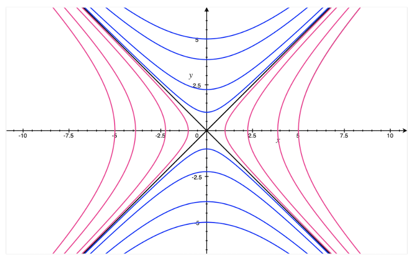
For example, $\{\begin{array}{l}{x}^{\prime }=y\\ y^{\prime }=x\end{array}$ has phase plane equation $\frac{dy}{dx}=\frac{x}{y}$. Separable: $ydy=xdx$, integrating gives $y^2/2=x^2/2+C$, or $y^2-x^2=c$. Trajectories are hyperbolas.

Equilibria

An equilibrium of an autonomous system is a state ${\mathbf{x}}^{\ast }$ where $\mathbf{F}({\mathbf{x}}^{\ast })=0$ — the rate of change is zero. Once at equilibrium, the system stays there.

Equilibria are also called critical points or fixed points. The phase plane equation $dy/dx=g/f$ is undefined at equilibria (both numerator and denominator are zero), so they appear as singular points in the phase portrait.

For a linear system ${\mathbf{x}}^{\prime }=A\mathbf{x}$, the origin is always an equilibrium (since $A\cdot 0=0$). If $\det A\ne 0$, the origin is the only equilibrium.

For nonlinear systems, equilibria can be anywhere — find them by solving $\mathbf{F}(\mathbf{x})=0$.

Why we care about equilibria

The long-term behavior of trajectories is dictated by which equilibria they approach (or avoid). Stable equilibria attract nearby trajectories; unstable ones repel. Mapping out equilibria and their stability gives a qualitative picture of the system’s dynamics without explicit solutions.

For the stability classification, see Stability of autonomous systems and Phase plane behaviour.

Autonomous form is canonical

A common technique: any non-autonomous system ${\mathbf{x}}^{\prime }=\mathbf{F}(t,\mathbf{x})$ can be made autonomous by introducing $t$ as an explicit state variable. Set $x_{n+1}=t$, $x_{n+1}^{\prime }=1$. Now the augmented system $(\mathbf{x},x_{n+1}{)}^{\prime }=(\mathbf{F}(x_{n+1},\mathbf{x}),1)$ is autonomous in $(n+1)$-dimensional state space.

This shows there’s no loss of generality in studying autonomous systems — but autonomous systems in their natural number of dimensions are usually easier to analyze.

For the linear special case, see Linear autonomous system. For visualizing trajectories, see Phase plane behaviour.