A line graph is the right tool when the x-axis is continuous: adjacent points are meaningfully connected, and the direction and rate of change matter. Time-series, trends, anything that varies smoothly. Vehicle velocity over time, with one line per vehicle, is a line graph.
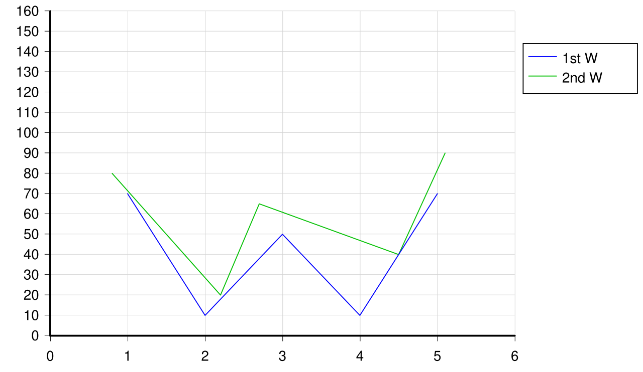 Image: Simple line chart, CC BY-SA 3.0
Line graphs make trends easier to see than scatter plots do, because connecting the points emphasizes the direction. They also handle multiple series well, with one line per series and a legend identifying each.
A common failure mode: a line graph with too few points starts to look like a polyline drawn through arbitrary corners, and the eye over-interprets the angles. With three or four points, a Bar chart or Scatter plot is often clearer.
The defining contrast with scatter plots is the connecting line. Scatter plots leave the points disconnected, which is right when adjacent doesn’t mean anything in particular. Line graphs connect them, which is right when adjacent does mean something: successive points represent the same phenomenon at successive times or successive values of some continuous parameter.
The raw ECG signal is the canonical example: voltage indexed by continuous time, drawn as a line connecting successive samples. So is any sensor trace, any stock price over time, any temperature reading. The shape of the curve carries information about the rate of change, the periodicity, the local maxima and minima, all of which a line graph displays at a glance.
For very dense data (an ECG sampled at 500 Hz, a one-minute recording is 30,000 points), the line can become visually busy. Subsampling, smoothing with a Moving-average filter, or showing only a representative window are all common responses.
In Matplotlib, ax.plot(x, y) draws a line graph. The third argument is a format string ('r-' for red solid, 'b--' for blue dashed, 'g^-' for green triangles connected by lines).