The moving-average filter is the simplest smoothing tool for reducing High-frequency noise. It does exactly what the name says.
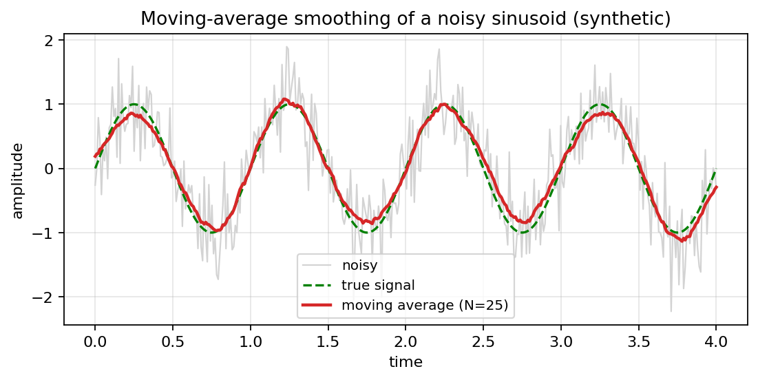 Noisy sinusoid (gray) smoothed by an moving-average filter (red). True signal in dashed green.
Pick a window size , usually an odd number. Slide the window along the signal sample by sample. At each position, compute the average of the samples currently inside the window, and set that average as the output sample at the corresponding position. Move the window forward one sample. Repeat. The output signal, the moving average, is a smoothed version of the input.
Why does this reduce noise? It’s the law of large numbers applied locally. If the noise at each sample is roughly random, equally likely to push the value up or down, then averaging samples lets the upward and downward pushes mostly cancel. A noisy sample at the center of the window gets pulled toward the average of its neighbors, which is closer to the true underlying signal. The slow features of the real signal pass through almost unchanged, because all samples in the window agree about them. The fast fluctuations cancel; the slow trend survives.
The tradeoff
There’s a tradeoff embedded in the choice of :
- A small window () barely smooths the signal. Only the very fastest fluctuations get averaged out.
- A large window () smooths much more aggressively. Noise is greatly reduced, but the moving average is also less responsive to genuine fast features, and sharp transitions get blurred.
The right is large enough to suppress the noise but small enough to preserve the features we care about. There are analytical methods for picking it (looking at the spectral content of the noise and the desired bandwidth) but for most engineering work, visual inspection suffices: try a few values of , plot the result, pick the one that visibly removes noise without losing features.
Causal delay
A moving-average filter, as described, has a delay. Two distinct issues:
- Fill delay. When we slide the window starting from sample 0, we don’t have enough data to fill the window until sample . The first outputs are undefined (Pandas writes
NaN). - Group delay. Even once the window is full, the filter’s output at time summarizes samples from through . Its effective time-center sits at the middle of the window, so a feature in the input shows up in the output shifted by samples. This is the group delay of the causal -point moving average, the same shift you’d see plotting the output on top of the input.
For real-time processing both delays matter; for offline analysis they matter less.
A centered moving average (window centered on the current sample, using neighbors on both sides) has zero group delay but isn’t causal: it requires future samples, which we don’t have at the moment of measurement.
In Pandas
The Pandas rolling method makes the filter a one-liner:
y_smoothed = y_with_noise_df.rolling(window=N).mean()The output is a Pandas Series of the same length as the input, with the first entries as NaN (the window doesn’t have enough samples to compute an average yet). This is the standard Python idiom for moving averages and is much faster than writing the loop ourselves, since the Pandas implementation is in compiled C.
The same rolling(...) machinery powers Feature extraction in the next stage of the preprocessing pipeline: rolling mean, std, max, Skewness, Kurtosis all use the same windowing logic.
Why it’s a low-pass filter
Formally the -point moving average is the FIR filter
with all taps equal to . Its frequency response is a (normalized) sinc, magnitude for sample rate . Low frequencies pass through nearly unattenuated; high frequencies get scaled toward zero. The first null of the response is at , and the −3 dB cutoff sits somewhat below that (roughly for an ideal -tap MA, from Smith’s DSP guide). So is a useful rough estimate of the corner: quick to compute, slightly optimistic. The response isn’t monotonic past the first null; the sinc has sidelobes that let some high-frequency content through. For aggressive high-frequency suppression with a flat passband, designed FIR filters or IIR filters (Butterworth, Chebyshev) do better, left for later signal-processing courses.