Exponential diode model

The exponential diode model uses the full Diode equation $i_D=I_S{e}^{v_D/V_T}$ as the diode’s $i$–$v$ relation, with no linearising approximation. It is the most accurate large-signal model and the least convenient to use, because combining the exponential with the rest of the circuit produces a transcendental equation that has no closed-form solution.

Where the transcendental equation comes from

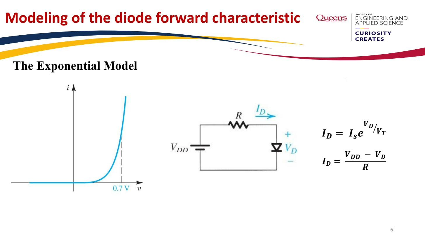
Take the worked circuit from the Constant-voltage-drop model: a supply $V_{DD}$, a series resistor $R$, and a diode. Kirchhoff’s voltage law gives

$V_{DD}=i_{D}R+v_D$

That is one equation in two unknowns ($i_D$, $v_D$). The second equation is the diode’s own characteristic:

$i_D=I_S{e}^{v_D/V_T}$

Substitute the diode equation into the KVL equation:

$V_{DD}=I_{S}R{e}^{v_D/V_T}+v_D$

Now $v_D$ appears both inside an exponential and outside it as a linear term. There is no algebraic rearrangement that isolates $v_D$ — this is a transcendental equation. You cannot write $v_D=(\text{something})$. The standard way out is Iterative diode analysis: guess, compute, refine, repeat until the value stops changing. A graphical “load-line” intersection (the diode curve crossed with the resistor’s straight line) is the same solution viewed geometrically.

Diode equation + KVL gives a transcendental equation, solved iteratively.

When it is worth it

Use the exponential model only when you need accuracy the Constant-voltage-drop model cannot give — for example when the answer depends sensitively on the exact diode voltage (precision references, log amplifiers, exponential temperature compensation), or when the diode current is far from the value at which “0.7 V” was calibrated. For ordinary rectifier and switching analysis the CVD model is close enough and the iteration is not worth the effort. This model is also the starting point for the Diode small-signal resistance: you differentiate this exponential at the operating point to get $r_d$.