Transmission line

A transmission line is a two-conductor structure that guides electromagnetic energy from a source to a load. Unlike a lumped-element circuit connection, the line itself has electrical effects: voltages and currents propagate along it as waves, with finite travel time. The line is a distributed network with its own propagation behavior.

Common physical forms:

• Coaxial cable: inner conductor + outer shield, dielectric between.
• Two-wire line: parallel wires, dielectric between (or air).
• Microstrip / stripline: PCB traces over a ground plane.
• Twin-lead: parallel ribbon, used historically for TV antennas.

For TEM-mode lines (the focus of Electromagnetics), the electric and magnetic fields are entirely transverse to the line — no field components along the propagation direction. This requires two conductors. Higher-order modes (single-conductor waveguides) are covered in later courses.

When transmission line effects matter

A rule of thumb: when the line length $l$ is at least 1% of a wavelength $\lambda$, transmission line effects can’t be ignored:

$\frac{l}{\lambda }\ge 0.01\Rightarrow \text{treat as TL}.$

At 60 Hz powerline frequency, $\lambda =5000$ km, and only intercontinental cables qualify. At 1 GHz, $\lambda =30$ cm — a PCB trace longer than 3 mm needs TL analysis. At 100 GHz, ~3 μm.

What goes wrong if you ignore TL effects? Two things:

1. Phase delay. Signals arrive at the load later than at the source: $V_{B{B}^{\prime }}(t)=V_{A{A}^{\prime }}(t-l/u_p)$. For a 1 kHz signal on a 20 km line, the phase shift is significant.
2. Dispersion. Different frequency components travel at different speeds (in dispersive media), distorting pulses. High-speed digital signaling and long-haul fiber design hinges on this.

Phase delay

The total phase delay between input (at $z=0$) and output (at $z=l$) of a lossless line is

${\varphi }_{\text{delay}}=\beta l=\frac{\omega l}{u_p}=\frac{2\pi l}{\lambda }\text{(radians)}.$

A pure sinusoid at frequency $\omega$ entering at $z=0$ exits at $z=l$ delayed by $\beta l$ in phase — equivalently, a time delay $t_d=l/u_p$. For a 30 cm coax with $u_p=0.66c$, the delay is $t_d=0.3/(0.66\cdot 3\times 10^8)\approx 1.5$ ns.

Phase delay is the bookkeeping of “how late does the output sinusoid lag the input sinusoid?” For a non-dispersive line, this delay is the same for every frequency, so a pulse arrives delayed but undistorted. For a dispersive line, phase delay varies with frequency — different components arrive shifted by different amounts, and the pulse spreads.

Phase delay is distinct from propagation delay (the time-of-flight of a wave front, $l/u_p$, identical to phase delay in the non-dispersive case) and from group delay ($l/u_g$, the time-of-flight of a pulse envelope, equal to phase delay only in non-dispersive media). In a non-dispersive line, all three coincide. In a dispersive medium, they differ — phase delay still describes the steady-state sinusoidal delay, but the energy and information in a pulse travel at the group velocity.

Dispersion

A line is dispersive when the Phase velocity $u_p=\omega /\beta$ depends on frequency. Equivalently, $\beta (\omega )$ is not strictly linear in $\omega$.

In an ideal lossless TEM line, $\beta =\omega \sqrt{L^{\prime }{C}^{\prime }}$ is exactly linear in $\omega$, and $u_p$ is constant. No dispersion. A pulse keeps its shape as it propagates — every Fourier component travels at the same speed.

Real lines deviate from the ideal in three ways:

1. Conductor loss with frequency dependence: $R^{\prime }(\omega )$ rises as $\sqrt{\omega }$ from skin effect, making $\gamma$ deviate from $j\omega \sqrt{L^{\prime }{C}^{\prime }}$. This contributes mild dispersion at high frequencies.
2. Dielectric loss: $G^{\prime }(\omega )$ and the frequency-dependent dielectric permittivity introduce dispersion in lossy lines.
3. Multi-mode / waveguide effects: above certain frequencies, higher-order modes (TE, TM) can co-propagate with the TEM mode, each with its own $u_p$. Microstrip has small TE/TM contamination that increases with frequency (“quasi-TEM”).

Consequences of dispersion:

• Pulse spreading. A short pulse contains a wide band of frequencies. If they propagate at different speeds, the pulse smears in time. For a fiber-optic cable carrying 100 Gb/s, dispersion is the dominant limit on link distance.
• Group velocity $u_g=d\omega /d\beta$ becomes the relevant “signal speed” instead of $u_p$. In normal dispersion (positive $d{u}_p/d\omega$), low frequencies travel faster than high — chirp. In anomalous dispersion (negative), the reverse.
• Phase velocity can exceed $c$ in dispersive media without violating relativity, because phase velocity isn’t the speed of information transport.

In Electromagnetics, the dispersion-free lossless line is the working model. Dispersion proper is treated in later wave-propagation and fiber-optics courses, where the dispersion relation $\omega (\beta )$ and group velocity become the central tools.

Lumped-element model

A short segment of length $\Delta z$ of any TEM line can be modeled as a series RL plus a shunt GC, all per unit length:

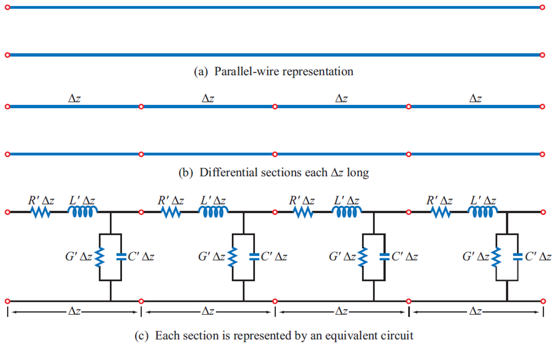
• $R^{\prime }$ (Ω/m): combined resistance of both conductors per unit length.
• $L^{\prime }$ (H/m): combined inductance of both conductors per unit length.
• $G^{\prime }$ (S/m): conductance through the dielectric per unit length.
• $C^{\prime }$ (F/m): capacitance between the conductors per unit length.

These four parameters depend on the line’s geometry and material. For a coaxial line with inner/outer radii $a,b$ and dielectric $ϵ,\mu ,\sigma$:

$L^{\prime }=\frac{\mu }{2\pi }\ln \frac{b}{a},C^{\prime }=\frac{2\pi ϵ}{\ln (b/a)},G^{\prime }=\frac{2\pi \sigma }{\ln (b/a)},R^{\prime }=\frac{R_s}{2\pi }\left(\frac{1}{a}+\frac{1}{b}\right).$

Two universal relations follow:

$L^{\prime }{C}^{\prime }=\mu ϵ,\frac{G^{\prime }}{C^{\prime }}=\frac{\sigma }{ϵ}.$

These hold for any TEM line. They reduce the four parameters to effectively two independent ones once geometry is fixed.

Telegrapher’s equations

Applying KVL and KCL to the $\Delta z$ segment and taking $\Delta z\to 0$:

$-\frac{\partial v}{\partial z}=R^{\prime }i+L^{\prime }\frac{\partial i}{\partial t},$ $-\frac{\partial i}{\partial z}=G^{\prime }v+C^{\prime }\frac{\partial v}{\partial t}.$

These are the telegrapher’s equations — coupled PDEs for $v(z,t),i(z,t)$. See Telegrapher’s equations.

In phasor form (sinusoidal steady state), ${\partial }_t\to j\omega$:

$-\frac{d\tilde{V}}{dz}=(R^{\prime }+j\omega L^{\prime })\tilde{I},$ $-\frac{d\tilde{I}}{dz}=(G^{\prime }+j\omega C^{\prime })\tilde{V}.$

Decouple by differentiating again:

$\frac{d^2\tilde{V}}{d{z}^2}={\gamma }^2\tilde{V},\frac{d^2\tilde{I}}{d{z}^2}={\gamma }^2\tilde{I},$

with propagation constant

$\gamma =\sqrt{(R^{\prime }+j\omega L^{\prime })(G^{\prime }+j\omega C^{\prime })}=\alpha +j\beta .$

These are 1D wave equations. Solutions: forward and backward propagating waves $e^{\pm \gamma z}$.

Characteristic impedance

The ratio of voltage to current for a single forward-propagating wave is the Characteristic impedance:

$Z_0=\sqrt{\frac{R^{\prime }+j\omega L^{\prime }}{G^{\prime }+j\omega C^{\prime }}}.$

For a lossless line ($R^{\prime }=G^{\prime }=0$): $Z_0=\sqrt{L^{\prime }/C^{\prime }}$ — real-valued. Common standard values: 50 Ω (RF coax), 75 Ω (TV cable), 110 Ω (twisted pair).

$Z_0$ depends only on line geometry and dielectric — not on length, not on what’s connected. It’s the intrinsic impedance of the line for traveling waves.

Lossless line

The common idealization $R^{\prime }=G^{\prime }=0$. Then:

$\gamma =j\omega \sqrt{L^{\prime }{C}^{\prime }}=j\omega \sqrt{\mu ϵ}=j\beta ,\alpha =0.$

Phase velocity:

$u_p=\frac{\omega }{\beta }=\frac{1}{\sqrt{L^{\prime }{C}^{\prime }}}=\frac{1}{\sqrt{\mu ϵ}}=\frac{c}{\sqrt{{ϵ}_r}}.$

For a non-magnetic dielectric, the wave moves at $c$ scaled down by $\sqrt{{ϵ}_r}$. A typical coax with ${ϵ}_r\approx 2.3$ has $u_p\approx 0.66c$.

Wavelength on the line:

$\lambda =\frac{u_p}{f}=\frac{{\lambda }_0}{\sqrt{{ϵ}_r}},$

shorter than free-space wavelength by $\sqrt{{ϵ}_r}$. This is why a “quarter-wave” PCB stub is physically shorter than ${\lambda }_0/4$.

What lives on the line

Two waves coexist: forward $V_0^{+}{e}^{-\gamma z}$ and backward $V_0^{-}{e}^{+\gamma z}$. Total voltage:

$\tilde{V}(z)=V_0^{+}{e}^{-\gamma z}+V_0^{-}{e}^{+\gamma z}.$

For lossless ($\gamma =j\beta$):

$\tilde{V}(z)=V_0^{+}{e}^{-j\beta z}+V_0^{-}{e}^{+j\beta z}.$

The backward wave is what an impedance mismatch at the load produces — see Reflection coefficient. When the load matches the line ($Z_L=Z_0$), $V_0^{-}=0$ and the line carries only a forward wave.