Spanning tree

A spanning tree of a connected, undirected Graph $G$ is a tree (a connected, acyclic subgraph) that includes every vertex of $G$.

Formally: given $G=(V,E)$, a spanning tree is a subgraph $T=(V^{\prime },E^{\prime })$ where:

• $V^{\prime }=V$ — same vertex set.
• $T$ is connected.
• $T$ is acyclic.

Since a tree on $n$ vertices has exactly $n-1$ edges, a spanning tree has $|V|-1$ edges from the original graph.

Subgraph

First, a definition: a subgraph of $G=(V,E)$ is any graph $G^{\prime }=(V^{\prime },E^{\prime })$ where $V^{\prime }\subseteq V$ and $E^{\prime }\subseteq E$. So $G^{\prime }$ uses some (or all) of $G$‘s vertices and some (or all) of its edges.

A spanning tree is a special kind of subgraph: it uses all the vertices, picks $|V|-1$ edges, and the result must be a tree.

Multiple spanning trees

Any graph has many possible spanning trees — different choices of which $|V|-1$ edges to include give different trees. The number can be huge: a complete graph on $n$ vertices has $n^{n-2}$ spanning trees (Cayley’s formula).

Minimum spanning tree (MST)

A minimum spanning tree is a spanning tree of minimum total weight:

$\text{cost}(T)={\sum }_{(v,w)\in E^{\prime }}c(v,w)$

The MST is the cheapest way to connect every vertex while still being a tree.

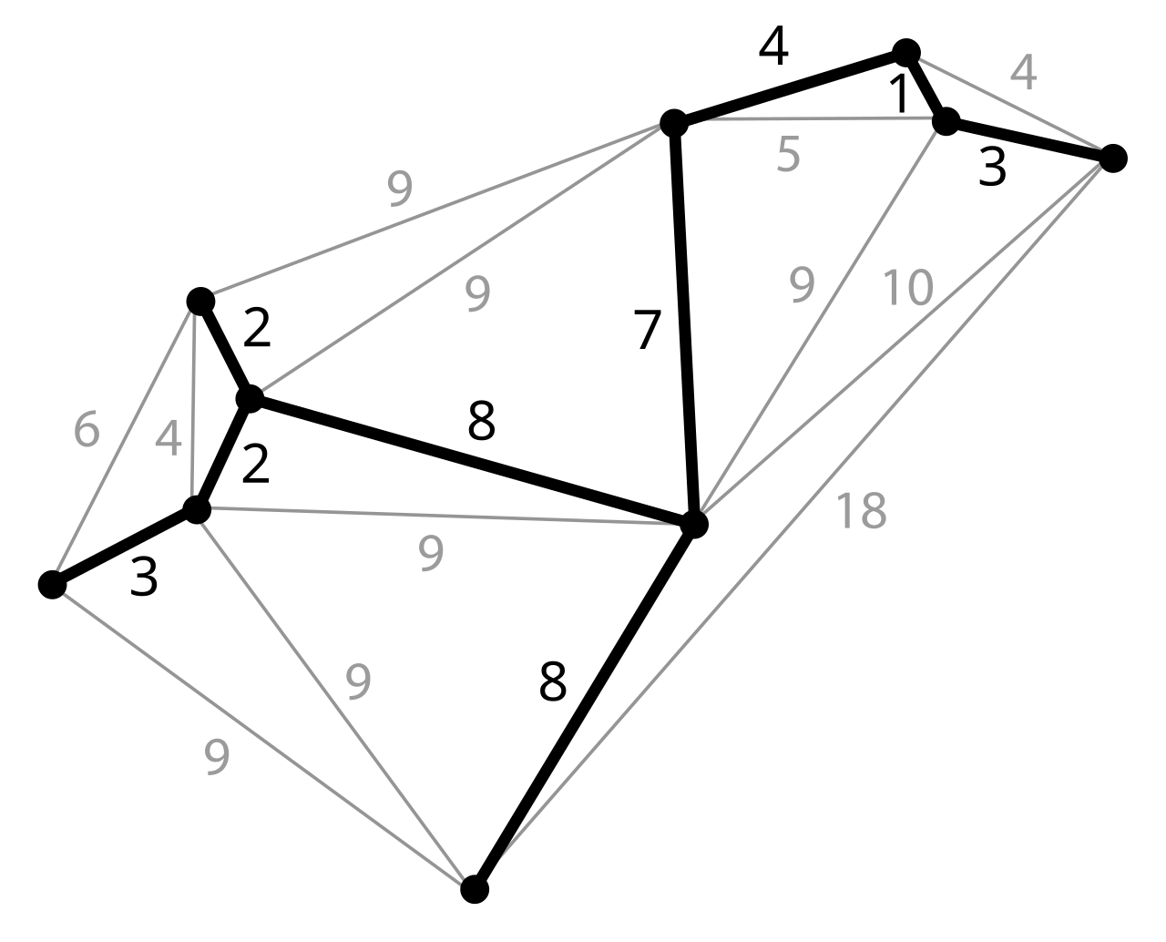Image: Minimum spanning tree, public domain — each point is a vertex; the highlighted edges form the spanning tree of minimum total length.

Why we want MSTs

Real-world applications:

• Network design: connect a set of houses with cable, minimizing total cable used.
• Cluster analysis: in machine learning, MSTs are used to identify clusters.
• Approximation algorithms: MSTs underlie approximation algorithms for the Traveling Salesman Problem.
• Image segmentation: connect similar regions in an image with minimum-weight edges.

Algorithms for MST

Two classic algorithms construct MSTs:

• Prim’s algorithm: grow a tree from a starting vertex, always adding the cheapest edge that connects to a new vertex. Greedy.
• Kruskal’s algorithm: sort all edges by weight, add the cheapest that doesn’t create a cycle. Also greedy.

Both are correct. Prim is easier to implement on dense graphs (like Dijkstra); Kruskal is easier on sparse graphs (just sort edges). Kruskal runs in $O(E\log E)=O(E\log V)$ (the equality holds because $E\le V^2$, so $\log E\le 2\log V$). Prim’s complexity depends on the priority queue: with a binary heap it’s $O((V+E)\log V)$, with a Fibonacci heap $O(E+V\log V)$. For connected graphs $E\ge V-1$, so $(V+E)\log V=\Theta (E\log V)$ — the two are asymptotically equivalent in that case. See Adjacency list for how the data structure choice interacts with the bound.

Spanning tree (without “minimum”)

Without the weight constraint, a spanning tree is just any tree covering all vertices. Algorithms like BFS and DFS each implicitly produce a spanning tree:

• BFS spanning tree: edges in the BFS forest, levels match BFS distance.
• DFS spanning tree: tree edges in the DFS traversal.

Both have $|V|-1$ edges and connect all reachable vertices.

For the standard greedy MST algorithm, see Prim’s algorithm. For graphs in general, see Graph.

Worked example

Consider a weighted undirected graph on six vertices A–F with edges AB(2), AC(3), BD(4), CD(1), CE(5), DF(6), EF(2) — the number in parentheses is each edge’s weight. Total weight of all edges: 23.

A spanning tree must include all 6 vertices and exactly 5 edges. Many possibilities; let’s find the minimum one.

Apply Kruskal’s algorithm:

1. Sort edges by weight: CD(1), AB(2), EF(2), AC(3), BD(4), CE(5), DF(6).
2. Add cheapest edge that doesn’t form a cycle:
   • CD(1) ✓ (no cycle yet).
   • AB(2) ✓.
   • EF(2) ✓.
   • AC(3) ✓ (connects {A,B} component to {C,D}).
   • BD(4) ✗ (creates cycle A-B-D-C-A).
   • CE(5) ✓ (connects {A,B,C,D} to {E,F}).
3. Stop: 5 edges chosen, all vertices connected.

MST: {AB, CD, EF, AC, CE}. Total weight: $2+1+2+3+5=13$.

The same MST results from Prim’s starting at any vertex:

• Start at A. Cheapest edge from {A}: AB(2). Add B.
• Cheapest from {A,B}: AC(3). Add C.
• Cheapest from {A,B,C}: CD(1). Add D.
• Cheapest from {A,B,C,D}: CE(5). Add E.
• Cheapest from {A,B,C,D,E}: EF(2). Add F.

Same MST.

Properties

A few key properties of MSTs:

1. Cut property: for any partition (cut) of the vertices into two non-empty sets, the minimum-weight edge crossing the cut is in some MST. (This is what makes Kruskal’s and Prim’s correct — at each step they include such a crossing edge.)

2. Cycle property: in any cycle, the heaviest-weight edge is not in any MST. (You could always swap it for a lighter edge that still keeps the tree connected.)

3. Uniqueness: if all edge weights are distinct, the MST is unique. With ties, multiple MSTs may exist (all with the same total weight).

Counting spanning trees

For a complete graph $K_n$ (every pair of vertices connected), the number of spanning trees is

$\tau (K_n)=n^{n-2}$

This is Cayley’s formula (1889). For $n=4$: $4^2=16$ spanning trees. For $n=10$: $10^8$ = 100 million.

For arbitrary graphs, the Matrix Tree Theorem gives a formula via the Laplacian matrix’s eigenvalues — but it’s mostly of theoretical interest. In practice, you compute one MST, not enumerate all spanning trees.

Variations

• Maximum spanning tree: opposite of minimum — find the costliest spanning tree. Same algorithms work with sign-flipped weights.
• Bottleneck spanning tree: minimize the maximum edge weight (rather than total weight). Different algorithm but related.
• Steiner tree: connect a subset of “required” vertices using any other vertices as helpers. NP-hard, doesn’t reduce to MST.
• Minimum spanning forest: for disconnected graphs, find an MST per component.

For the algorithms that actually compute MSTs, see Prim’s algorithm (and Kruskal’s, mentioned briefly above). For graph fundamentals, see Graph.