The Smith chart reads off impedance, admittance, and reflection coefficients in transmission-line theory and RF work. The chart is the image of the right half of the impedance plane under the Möbius transformation
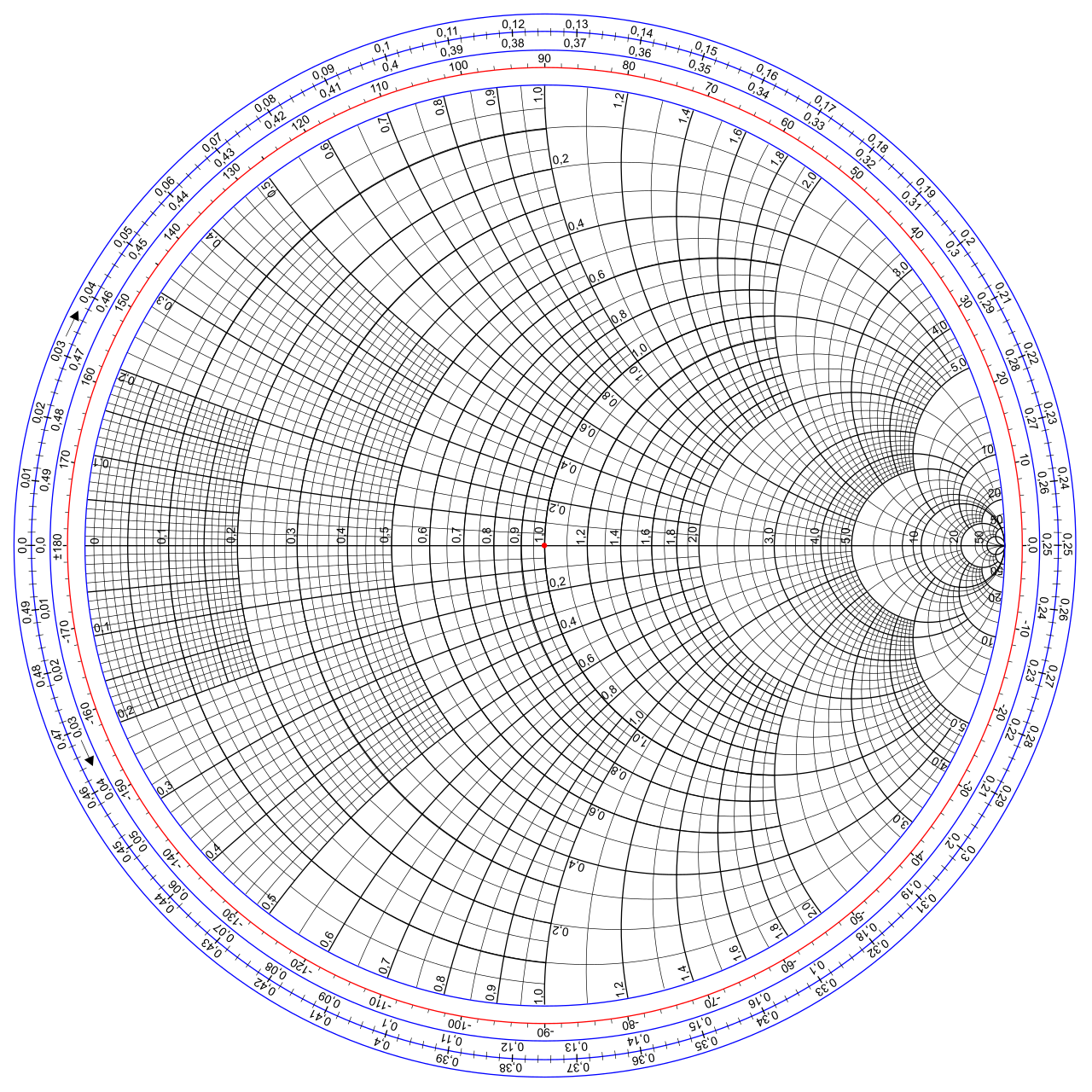 Image: Smith chart (generic), CC BY-SA 3.0. Constant-resistance circles and constant-reactance arcs.
Here is the load impedance, is the characteristic impedance of the transmission line, and is the reflection coefficient. Normalizing :
For passive loads (), , so lies in the unit disk of the complex plane.
The transformation
The map is a Möbius transformation. It maps:
- The right half-plane to the open unit disk .
- The imaginary axis to the unit circle .
- (matched load) to (no reflection, the center of the chart).
- (short circuit) to .
- (open circuit) to .
- (purely inductive) to (top of unit circle).
- (purely capacitive) to (bottom).
The curved grid
Because Möbius transformations send circles and lines to circles and lines, the rectangular grid of constant-resistance lines and constant-reactance lines in the -plane maps to a curved grid in the -plane:
- Constant resistance : maps to a circle in the -plane, tangent to the unit circle at . The tangency at happens because the open-circuit point lies on every vertical line (each such line is unbounded in the imaginary direction), and under the Möbius map. So every constant-resistance circle passes through (is tangent to the unit circle at) . Larger → smaller circle inside the unit disk, concentrating toward as and expanding to the full unit circle as .
- Constant reactance : maps to an arc of a circle passing through , for the same reason. Horizontal lines also pass through . The arc lies in the upper half-disk (positive reactance, inductive) or lower half-disk (negative reactance, capacitive), depending on the sign of .
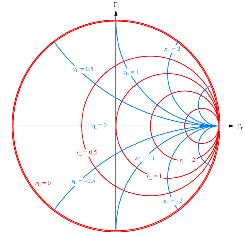 The two curved families of the grid: constant- circles (closed loops all tangent to ) and constant- arcs (open arcs running from out to the unit circle). Their intersection is the impedance point.
The two families of curves intersect at right angles, by Conformality (Möbius transformations are conformal away from their pole; the pole is at , outside the right half-plane).
What the chart lets you do
- Plot a load : find the intersection of the constant- circle and the constant- arc.
- Read the reflection coefficient directly: is the distance from the chart center; is the angle.
- Trace impedance along the transmission line: moving toward the source or load along a uniform line rotates around the chart center by an angle proportional to the electrical distance traveled.
- Design impedance-matching networks graphically: where to place stubs, series elements, etc., to move from a starting impedance to a target.
These days the chart mostly shows up as a visualization built into network analyzers and simulators, but the math behind it (Möbius transformation, conformal mapping, circles-to-circles) is what makes it work.
Applied workflow (Electromagnetics)
In a transmission-line context, the chart is used as a graphical calculator for impedance, admittance, Reflection coefficient, SWR, and matching network design.
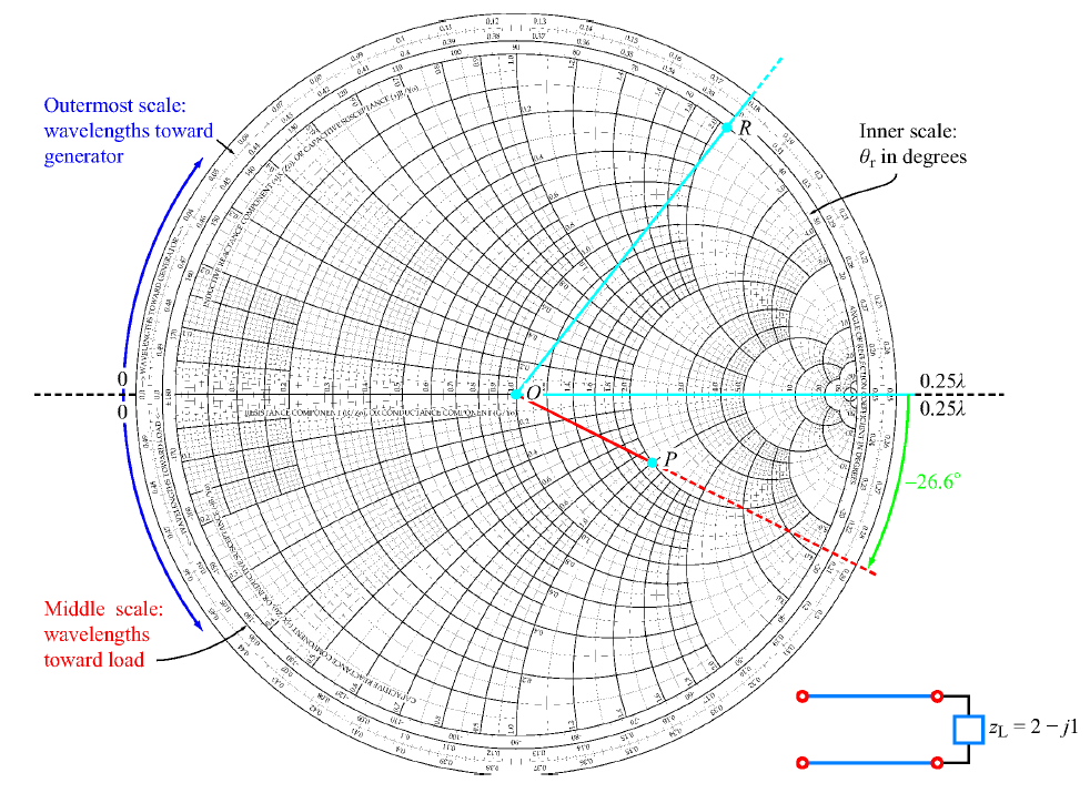
The chart has three scales around its rim:
- Inner scale: angle of reflection coefficient, in degrees.
- Middle scale: “wavelengths toward load” (WTL), distance from a reference point in , moving from the generator toward the load.
- Outer scale: “wavelengths toward generator” (WTG), distance moving from the load toward the generator.
Why the rim scales: moving along the line shifts the phase of . Moving a distance toward the generator multiplies by , a clockwise rotation around the chart center by radians. One full lap is .
Application 1: Find Γ from a load
Given normalized load :
- Find the intersection of the resistance circle and the reactance arc. Mark the point on the chart.
- is the distance from chart center to the point, divided by the distance from center to the rim ( circle).
- is read directly off the angle scale.
Example: gives , .
Application 2: Find wave impedance Z(d)
Given and want at distance from the load:
- Plot on the chart (point ).
- Draw the constant-SWR circle through , centered at the chart center. All wave impedances along the line lie on this circle.
- Rotate clockwise (toward generator) by as read from the outer scale. Land at point .
- Read from the intersecting resistance/reactance curves at .
For input impedance, rotate by the full electrical length .
Application 3: Find SWR
- Plot , draw constant-SWR circle.
- Where the SWR circle crosses the real axis to the right of origin (with ): that value of equals the SWR.
This works because on the real axis, is real, and at the right intersection (positive). The normalized impedance there is .
Application 4: Find voltage maxima/minima positions
The voltage maximum on the line occurs where (real, equal to SWR), the right intersection of the SWR circle with the axis.
To find (distance from load to first voltage maximum):
- Plot .
- Read the WTG scale at the angular position of .
- Move clockwise to the right- intersection; read the WTG scale there.
- Difference (mod ) is .
Voltage minimum is exactly farther: .
Application 5: Single-stub matching
- Plot normalized load admittance . (On the chart, is the point diametrically opposite, rotate 180°.)
- Move along the constant-SWR circle (toward generator) until you intersect the circle. Two intersections; pick one. Read off from the WTG scale.
- At that intersection point, the normalized admittance is . Need to cancel with a stub providing .
- For a short-circuited stub of : enter the chart at the “short” point (, the rightmost point on circle), move toward the generator along the rim until you reach a normalized admittance of . The distance traveled is the stub length .
- For an open-circuited stub: enter at the “open” point (, leftmost on ) and proceed similarly.
Placing the stub at distance from the load with length then makes the feedline see , matched.
Worked example
A 50 Ω line terminated in Ω. Normalize: .
- Plot on the chart at the intersection of and .
- , , read off.
- SWR from where constant-SWR circle hits real axis.
- , .
- For a -long line, rotate clockwise by (i.e., on the chart). New point gives .
In context
The Smith chart is the standard engineering application of Möbius transformations and conformal mapping. It’s why transmission-line theory leans on complex analysis: the impedance matching problem in -space is hard, but in -space it’s geometric. Move points around inside a disk, rotate along the line, read off matching conditions visually.
See Impedance matching for the applied use.