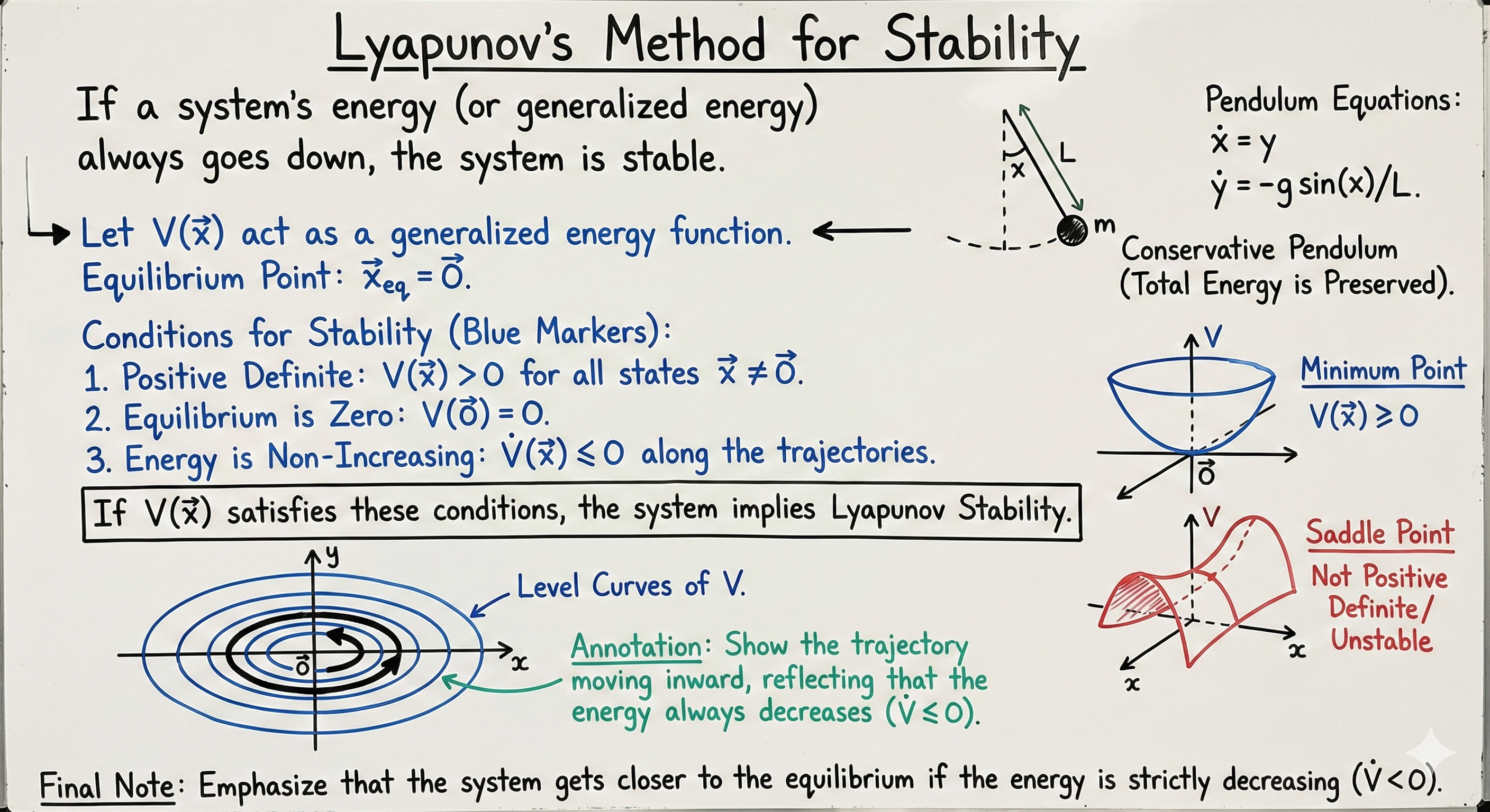
Lyapunov's method

Lyapunov’s method is a way to determine stability of an equilibrium without solving the ODE — by finding a scalar function $V(\mathbf{x})$ that behaves like an energy, and showing it never increases along solution trajectories. If energy decreases, the system runs out of energy and settles down at the equilibrium.

The method is especially powerful when linearization fails (eigenvalues on the imaginary axis), where linear theory is inconclusive.

Conceptual basis

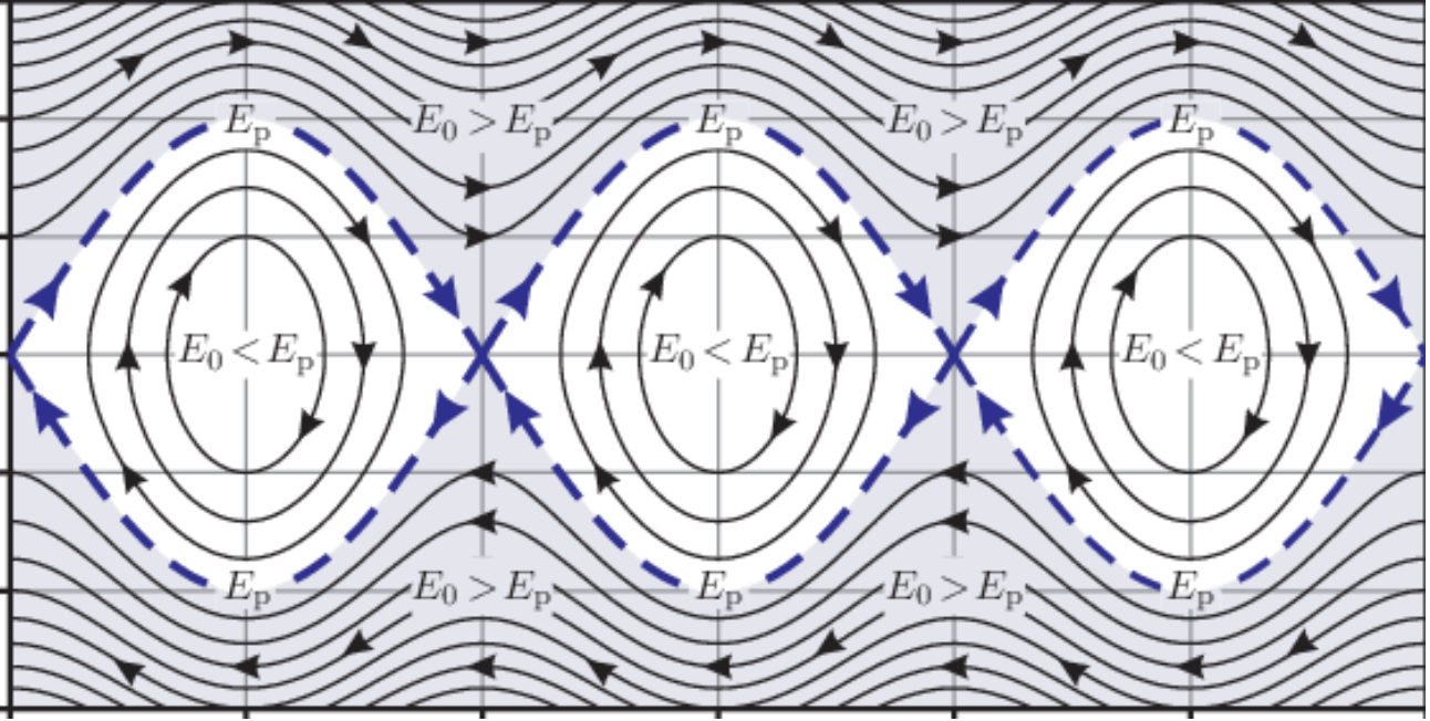
A conservative pendulum has its total energy preserved (no friction, no external forces). Solutions trace level curves of the energy function $E(\mathbf{x})$ — closed orbits at constant energy. The equilibrium has minimum energy.

If the pendulum has friction, energy decreases over time. Solutions spiral inward through level curves toward the equilibrium of minimum energy. This is asymptotic stability.

Lyapunov realized: any function $V(\mathbf{x})$ that has a minimum at the equilibrium and never increases along trajectories will play the same role as energy. The system “runs downhill” in $V$ until it reaches the minimum.

Definitions

A function $V(\mathbf{x})$ defined on a neighborhood $D$ of the equilibrium $0$ is:

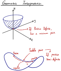
• Positive definite on $D$ if $V(0)=0$ and $V(\mathbf{x})>0$ for all $\mathbf{x}\in D\setminus \{0\}$.
• Positive semi-definite if $V(0)=0$ and $V(\mathbf{x})\ge 0$ for all $\mathbf{x}\in D$.
• Negative definite if $-V$ is positive definite.
• Negative semi-definite if $-V$ is positive semi-definite.

A typical positive-definite $V$ has a “bowl” shape with the bottom at $0$:

The derivative along trajectories

The key quantity is the time derivative of $V$ along solutions:

$\dot{V}(\mathbf{x}):=\frac{d}{dt}V(\mathbf{x}(t))=\nabla V\cdot {\mathbf{x}}^{\prime }(t)=\nabla V\cdot \mathbf{F}(\mathbf{x})$

You don’t need to know $\mathbf{x}(t)$ — just compute the gradient of $V$ and dot with $\mathbf{F}$. This is the rate of change of $V$ along whatever trajectory passes through $\mathbf{x}$.

If $\dot{V}<0$ everywhere (except at the equilibrium), $V$ strictly decreases on every trajectory — the system runs downhill in $V$, eventually reaching the bottom of the bowl.

Lyapunov stability theorem

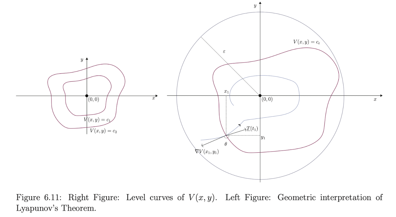
Let $0$ be an isolated critical point of ${\mathbf{x}}^{\prime }=\mathbf{F}(\mathbf{x})$, and $V$ be defined on a neighborhood $D$ of $0$ with $V$ positive definite on $D$. Then:

1. If $\dot{V}\le 0$ on $D$, then $0$ is stable.
2. If $\dot{V}<0$ on $D\setminus \{0\}$, then $0$ is asymptotically stable.

Strict negative definiteness of $\dot{V}$ implies asymptotic stability; semi-definite (allowing $\dot{V}=0$ on some set) only gives stability.

Lyapunov instability theorem

Suppose $V(0)=0$ and $V$ is defined on $D$ around the equilibrium. Then:

1. If for every disk around $0$ there exists a point where $V\ge 0$ and $\dot{V}>0$, then $0$ is unstable.
2. If for every disk around $0$ there exists a point where $V<0$ and $\dot{V}<0$, then $0$ is also unstable.

[Note: this specific claim is from general knowledge and hasn’t been independently verified. The standard Chetaev-style instability theorem requires the slightly stronger condition that the points have $V>0$ (strict) and $\dot{V}>0$ on a region adjacent to the equilibrium; some formulations allow $V\ge 0$ but require additional structure.]

The instability versions are about finding some direction in which $V$ grows — that direction’s trajectory escapes the equilibrium.

Worked example

Consider:

$\{\begin{array}{l}{x}^{\prime }=-x^3/2+2x{y}^3\\ y^{\prime }=-y^3\end{array}$

Linearization at origin: Jacobian is the zero matrix (all first derivatives vanish at origin) — so linear theory is useless.

Try a Lyapunov candidate: $V(x,y)=a{x}^2+b{y}^2$ for constants $a,b>0$.

• $V(0,0)=0$. ✓
• $V>0$ for $(x,y)\ne (0,0)$ when $a,b>0$. ✓ (positive definite)

Compute $\dot{V}$:

$\dot{V}=\frac{\partial V}{\partial x}(-x^3/2+2x{y}^3)+\frac{\partial V}{\partial y}(-y^3)$

$=2ax\cdot (-x^3/2+2x{y}^3)+2by\cdot (-y^3)$

$=-a{x}^4+4a{x}^2{y}^3-2b{y}^4$

For $\dot{V}<0$: substitute $u=x^2\ge 0$. Then $\dot{V}=-a{u}^2+4au{y}^3-2b{y}^4$.

Treat as quadratic in $u$: $-a{u}^2+4a{y}^{3}u-2b{y}^4$. Discriminant:

$D=(4a{y}^3{)}^2-4(-a)(-2b{y}^4)=16a^2{y}^6-8ab{y}^4=8a{y}^4(2a{y}^2-b)$

For the quadratic in $u$ (which opens downward since coefficient of $u^2$ is $-a<0$) to be always $\le 0$, we need its discriminant $\le 0$:

$8a{y}^4(2a{y}^2-b)\le 0$

Since $8a{y}^4\ge 0$, we need $2a{y}^2-b\le 0$, i.e., $b\ge 2a{y}^2$.

For this to hold for all $y$ in some neighborhood of $0$: $y$ is small, so $2a{y}^2$ is small, so any $b>0$ works for sufficiently small neighborhood. Specifically, $b>2a>0$ guarantees it on an open set around origin.

Conclusion: with $a=1,b=3$ (say), $V=x^2+3y^2$ is positive definite and $\dot{V}<0$ on a neighborhood of origin. By Lyapunov’s stability theorem, origin is asymptotically stable.

This is information linearization couldn’t provide.

Finding Lyapunov functions

There’s no general algorithm — finding a Lyapunov function is sometimes an art. Strategies:

1. For mechanical systems: try the total energy (kinetic + potential). Often works.
2. Quadratic Lyapunov function: $V(\mathbf{x})={\mathbf{x}}^{T}P\mathbf{x}$ for some positive definite matrix $P$. For linear systems, $\dot{V}={\mathbf{x}}^T(A^{T}P+PA)\mathbf{x}$, and you can solve the Lyapunov equation $A^{T}P+PA=-Q$ for a chosen $Q>0$.
3. Symmetric perturbations of energy: for nonlinear systems, modifications of the natural energy.
4. Use trajectory information if you’ve simulated: $V$ should decrease along observed trajectories.

For systems where the linear theory works, see Stability of autonomous systems. For the linearization technique, see Locally linear system.