The impulse response of a linear time-invariant (LTI) system is the system’s output when the input is a Dirac delta and the system is in its zero state (no stored energy at ). Equivalently, it’s the inverse Laplace transform of the system’s Transfer function :
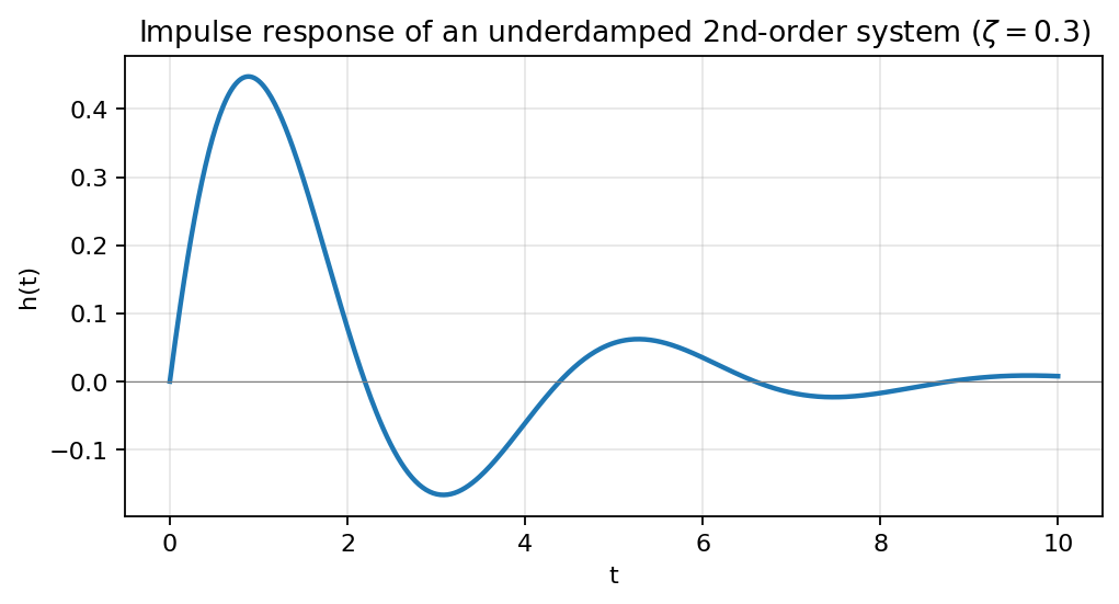 Impulse response of an underdamped second-order system, : exponentially damped oscillation.
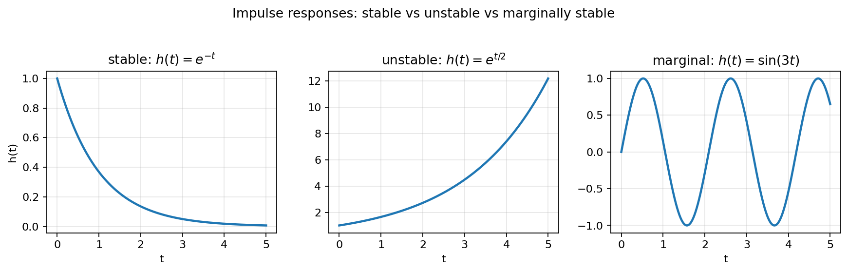 Three impulse responses: stable (decaying exponential), unstable (growing exponential), marginally stable (undamped sinusoid).
For a second-order linear ODE with zero initial conditions, the transfer function is , and the impulse response is
Why it matters
Once you know , you can compute the system’s response to any input via convolution:
This is the convolution form of the input-output relationship. The impulse response captures everything about how the system responds, the same way a transfer function does. They’re Laplace pairs.
Why “impulse”
If you input (a Dirac delta — an idealized instantaneous impulse), then , so , and .
So the impulse response is, literally, the system’s output when “kicked” with an idealized impulse.
Worked example
For the damped oscillator :
Transfer function: .
Complete the square: .
So .
Inverse Laplace using the shifted-sine form: .
So .
This is the system’s response to an impulse at . The factor is the damping; the is the underdamped oscillation.
In context
Two equivalent ways to compute system response:
- s-domain: , then inverse Laplace.
- Time domain: via convolution.
Both give the same answer. Method 1 is usually faster algebraically; method 2 is useful when is unwieldy or unknown in closed form.
The impulse response also makes physical sense: a complex system “smears” each input over time according to its impulse response. A short input gets stretched out (if the system is sluggish); a long input gets averaged (if the system has limited bandwidth).
Stability via impulse response
A system is bounded-input-bounded-output (BIBO) stable iff the impulse response is absolutely integrable. For a causal system (the standard case here, where for ):
The general statement uses , but for any causal LTI system the integrand is zero for negative , so the bound only needs to hold on . Use the lower limit that matches the system you’re analyzing.
For our LTI systems, this holds iff all poles of have strictly negative real parts.
Nonzero initial conditions
The transfer function and impulse response are defined for zero initial conditions. For nonzero initial conditions, the full solution is
where the second term is the homogeneous solution that handles the initial conditions:
Compute via the Characteristic equation separately, then add to the convolution result.
For example: , , .
Particular (zero IC): Laplace gives . Inverse: .
Homogeneous (nonzero IC): general . Apply , : , . So .
Full: .
Finding h(t) from a differential equation
For an LTI system defined by a linear constant-coefficient ODE
the impulse response is what comes out when . The technique splits into three time regions:
- : (causal system, zero input before the impulse). Also enforces causality.
- : satisfies the homogeneous equation. Find the characteristic roots ; write for .
- : integrate the ODE across the singularity (from to ). The integrals of bounded functions are zero; the integral of is 1; the integral of is the jump in , etc. This gives equations for the unknown constants.
Whether contains an impulse at depends on the relative orders vs : means no impulse component (Case 1); means an impulse at with some strength to determine (Case 2); is rare in practice.
This is the time-domain way to find . The s-domain approach is usually faster: write the transfer function algebraically and inverse-transform via Partial fraction decomposition.
Causality and stability from h(t)
For an LTI system, two of its properties can be read directly off the impulse response:
- Causal: for .
- BIBO stable: .
A causal signal with a factor is automatically the impulse response of a causal system. A signal that decays fast enough at is the impulse response of a stable system.