Hash table

A hash table stores key-value pairs and supports very fast lookup, insertion, and deletion — typically $O (1)$ on average. It implements the map (associative array, dictionary) abstract data type: given a key, retrieve the associated value.

The trick: a hash function converts each key into an array index (a “bucket”). To look up a value, you hash the key, jump to that bucket. No traversal needed.

The catch: the bucket might already be occupied by a different key — a collision. Every hash table design is essentially a strategy for handling collisions.

Map operations

The standard interface:

get(key) — return the value associated with the key, or NULL.
put(key, value) — insert a new entry, or replace the value if the key already exists.
remove(key) — delete the entry for the key (or do nothing if absent).
size(), isEmpty() — state queries.

Hash function

A hash function h takes a key and returns an integer in [0, M-1] where M is the table size. Simple example for integer keys:

$h (x) = x mod M$

For string keys, you’d combine the bytes somehow — sum them, multiply by primes, XOR them together. Real hash functions are more sophisticated (FNV, MurmurHash, SipHash) and try to spread keys uniformly across buckets.

int hashFunc(int idNum) {
    int ARRAY_SIZE = 100000;
    int bucket = idNum % ARRAY_SIZE;
    return bucket;
}

The name “hash” comes from the fact that the function “chops up and mixes” the key — like hashing meat into smaller pieces — to produce an index.

Collisions

When two different keys hash to the same bucket, that’s a collision. The pigeonhole principle guarantees collisions are inevitable for any non-trivial hash table — there are infinitely many possible keys but only $M$ buckets.

Two main strategies for handling collisions: closed hash tables (open addressing) and open hash tables (separate chaining).

Closed hash table (open addressing)

When a collision occurs, look for the next available bucket along a fixed probe sequence and store there. Three textbook schemes, each with its own atomic note:

Linear probing — step $f (i) = i$ . Simplest, best cache behaviour, suffers primary clustering.
Quadratic probing — step $f (i) = c_{1} i + c_{2} i^{2}$ . Eliminates primary clustering; secondary clustering remains.
Double hashing — step depends on a second hash $h_{2} (k)$ . Best probe count, closely approximates ideal uniform hashing; worst cache behaviour.

Probe-count summary

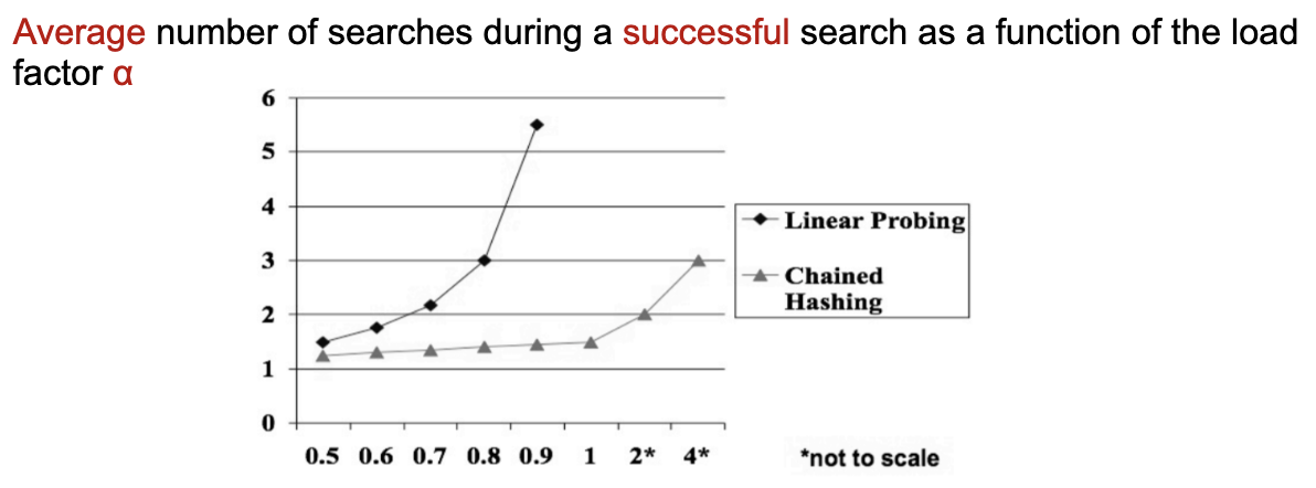
Define load factor $α = n / m$ where $n$ is items, $m$ is buckets. The four scheme behaviours at a glance:

Scheme	Unsuccessful (avg probes)	Successful (avg probes)
Uniform hashing (ideal)	$\frac{1}{1 - α}$	$\frac{1}{α} ln \frac{1}{1 - α}$
Double hashing	≈ uniform	≈ uniform
Quadratic probing	between uniform and linear	between
Linear probing	$\frac{1}{2} (1 + \frac{1}{( 1 - α ) ^{2}})$	$\frac{1}{2} (1 + \frac{1}{1 - α})$

The contrast is dramatic at high load. At $α = 0.9$ , uniform predicts ~10 probes for unsuccessful search; linear predicts ~50.5. So closed tables typically resize at $α = 0.7$ (textbook linear) to $α = 0.9$ (Robin Hood / SwissTable).

Deletion needs tombstones

For all open-addressing schemes, naively setting a deleted slot to NULL breaks the probe chain. The fix is a tombstone: a sentinel value lookups skip over but inserts may reuse. See Linear probing for the worked picture.

Pros (open-addressing in general): fixed-size storage, no per-entry pointers, good cache behaviour. Cons: needs spare capacity; performance degrades sharply as $α \to 1$ .

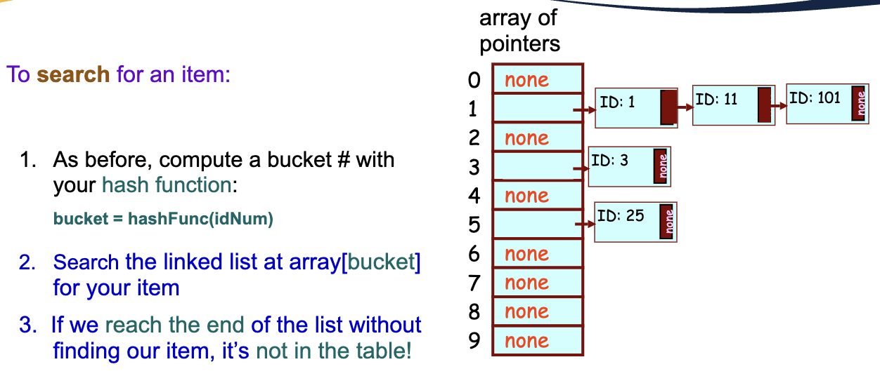
Open hash table (separate chaining)

Each bucket holds a Linked list (or another data structure) of all keys hashing to that bucket — see Separate chaining for the full treatment, including chain-as-tree variants and per-node memory overhead.

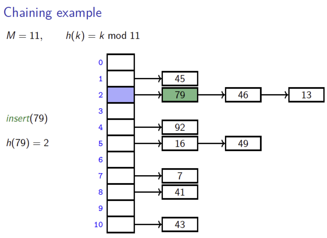
Quick analysis: average chain length $= α$ , so unsuccessful search is $Θ (1 + α)$ and successful is $Θ (1 + α /2)$ . Worst case $O (n)$ if every key collides — see hash flooding below.

Closed vs open

Closed (open addressing): faster average case for moderate load, better cache. Resize before $α$ approaches 1.
Open (chaining): handles dynamic load gracefully, simpler deletion, worse cache.

Modern languages mostly use open addressing for built-in hash maps: Python dict uses a perturbation-based probe, Rust’s std::collections::HashMap uses Google’s SwissTable design, and Go’s map uses bucketed open addressing (each bucket holds 8 slots searched linearly).

Worst case: O(n)

If many keys collide, both schemes degrade. In the worst case (every key hashes to one bucket), search is $O (n)$ .

With a good hash function on a typical workload, this worst case is rare in expectation. But adversarial workloads do happen in practice — particularly on the public-facing internet, where an attacker can craft requests with deliberately colliding keys.

Hash flooding

If a server uses a deterministic, public hash function for an attacker-controllable input (HTTP query parameters, JSON keys, form fields), the attacker can pick keys that all collide. Every insertion then walks the full chain, turning the supposedly $O (1)$ map operation into $O (n)$ , which compounds across $n$ insertions to $O (n^{2})$ wall-clock work for a single request. This is hash flooding.

The first widely-publicized hits were demonstrated against PHP, Java, Python, Ruby, Node.js, and others around 2011 (CVE-2011-4815 and related). A single ~2 MB POST body with crafted keys could pin a CPU for many seconds.

The defense is keyed hashing: hash with a per-process random seed (SipHash with a secret key, for example) so an attacker cannot predict which keys collide. Modern language runtimes — Python, Ruby, Rust’s default HashMap, Go’s map, Perl — all do this. Older systems and ad-hoc hash maps written by programmers who only read the average-case analysis are still vulnerable.

So hash tables aren’t unconditionally safer than BSTs: a BST has bad worst-case shape on sorted insertion (an accidental attacker), while a hash table has bad worst-case shape on adversarially chosen keys (an intentional attacker). Both deserve mitigation in production code.

Idriss Rami — Notes

Explorer