Dijkstra's algorithm

Dijkstra’s algorithm computes the shortest paths from a single source vertex to all other vertices in a weighted Graph with non-negative edge weights. The classic algorithm for “what’s the shortest route from A to B?” in a road network, network routing, or any shortest-path problem.

Constraints:

Graph is connected.
Edges can be directed or undirected.
Edge weights must be non-negative. (Negative weights need Bellman-Ford instead.)

The idea

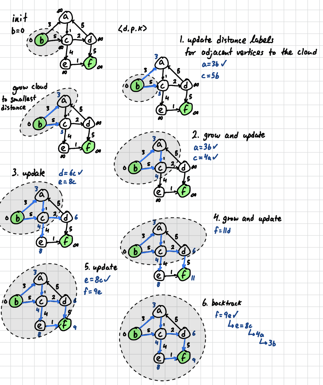
Grow a “cloud” of vertices whose shortest distances from the source are now known. Start with just the source. At each step, find the closest vertex outside the cloud, add it to the cloud, and update distance estimates for its neighbors.

Each vertex $u$ has three pieces of information:

distance $d (u)$ : best known distance from source to $u$ .
predecessor: the previous vertex on the shortest path to $u$ (lets you reconstruct the path).
flag: whether the shortest path to $u$ is finalized (in the cloud) or still tentative.

Algorithm

Initialize $d (source) = 0$ , $d (v) = \infty$ for all other $v$ .
Mark all vertices unvisited.
While there are unvisited vertices:
- Pick the unvisited vertex $z$ with the smallest tentative $d$ .
- Mark $z$ as visited.
- For each unvisited neighbor $u$ of $z$ , relax the edge $(z, u)$ : $d (u) \leftarrow min {d (u), d (z) + weight (z, u)}$
When done, $d (v)$ is the shortest path from source to $v$ .

Edge relaxation is the key step: for an edge $(u, z)$ where $z$ is not yet in the cloud, check if going through $u$ gives a better path to $z$ than what you currently have:

$d (z) \leftarrow min {d (z), d (u) + weight (e)}$

If yes, update.

Worked example

Find the shortest path from Providence (PVD) to Honolulu (HNL):

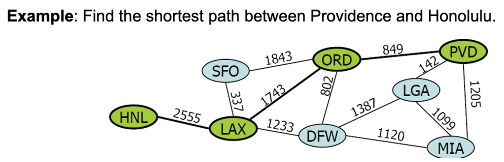
Bold edges form the resulting shortest path through the airport graph.

Implementation

void Dijkstra(int Graph[MAX][MAX], int n, int start) {
    int cost[MAX][MAX];
    int distance[MAX], pred[MAX], visited[MAX];
    
    // Build cost matrix; INFINITY for missing edges
    for (int i = 0; i < n; i++) {
        for (int j = 0; j < n; j++) {
            if (Graph[i][j] == 0)
                cost[i][j] = INFINITY;
            else
                cost[i][j] = Graph[i][j];
        }
    }
    
    // Initialize from start
    for (int i = 0; i < n; i++) {
        distance[i] = cost[start][i];
        pred[i]     = start;
        visited[i]  = 0;
    }
    distance[start] = 0;
    visited[start]  = 1;
    
    int count = 1;
    // We've already marked the start as visited, so we need to mark
    // n - 1 more vertices. Loop until count == n.
    while (count < n) {
        int mindistance = INFINITY;
        int nextnode;
        
        // Find the unvisited node with the smallest distance
        for (int i = 0; i < n; i++) {
            if (distance[i] < mindistance && !visited[i]) {
                mindistance = distance[i];
                nextnode    = i;
            }
        }
        
        visited[nextnode] = 1;
        
        // Relax edges from nextnode
        for (int i = 0; i < n; i++) {
            if (!visited[i]) {
                if (mindistance + cost[nextnode][i] < distance[i]) {
                    distance[i] = mindistance + cost[nextnode][i];
                    pred[i]     = nextnode;
                }
            }
        }
        count++;
    }
}

The pred[] array stores predecessors so you can reconstruct the shortest path: walk backward from a target through pred to the source.

Big O

The naïve implementation above is $O (V^{2})$ — for each iteration, scan all vertices to find the minimum-distance unvisited one.

With a priority queue (binary heap), it’s $O ((V + E) lo g V)$ — better for sparse graphs.

With a Fibonacci heap, $O (V lo g V + E)$ — theoretical best, rarely used in practice due to the constant factor.

Why non-negative weights only

The algorithm assumes that once a vertex is added to the cloud, its distance is finalized — no future iteration can find a shorter path. This holds when all edges are non-negative. If negative edges exist, you might find a shorter path later by going through a not-yet-finalized vertex. Use Bellman-Ford for that.

Use cases

Road navigation. Google Maps and similar use Dijkstra (or its variants like A*).
Network routing. OSPF (Open Shortest Path First) uses Dijkstra to compute routing tables.
Game AI. Pathfinding in grid worlds.
Airline flights. Finding cheapest connections across hubs.

The output is the shortest distance from the source to every vertex — even if you only care about one target, the algorithm computes them all. For pure single-pair queries, A* (a heuristic-guided variant) is often faster.

For finding the minimum-weight tree connecting all vertices, see Prim’s algorithm — a similar greedy approach but for spanning trees.

Idriss Rami — Notes

Explorer