Binary tree

A binary tree is a tree where every node has at most two children — conventionally called the left child and the right child. The two-child constraint makes binary trees particularly easy to reason about and to implement, and they form the basis for BSTs, AVL trees, red-black trees, and heaps.

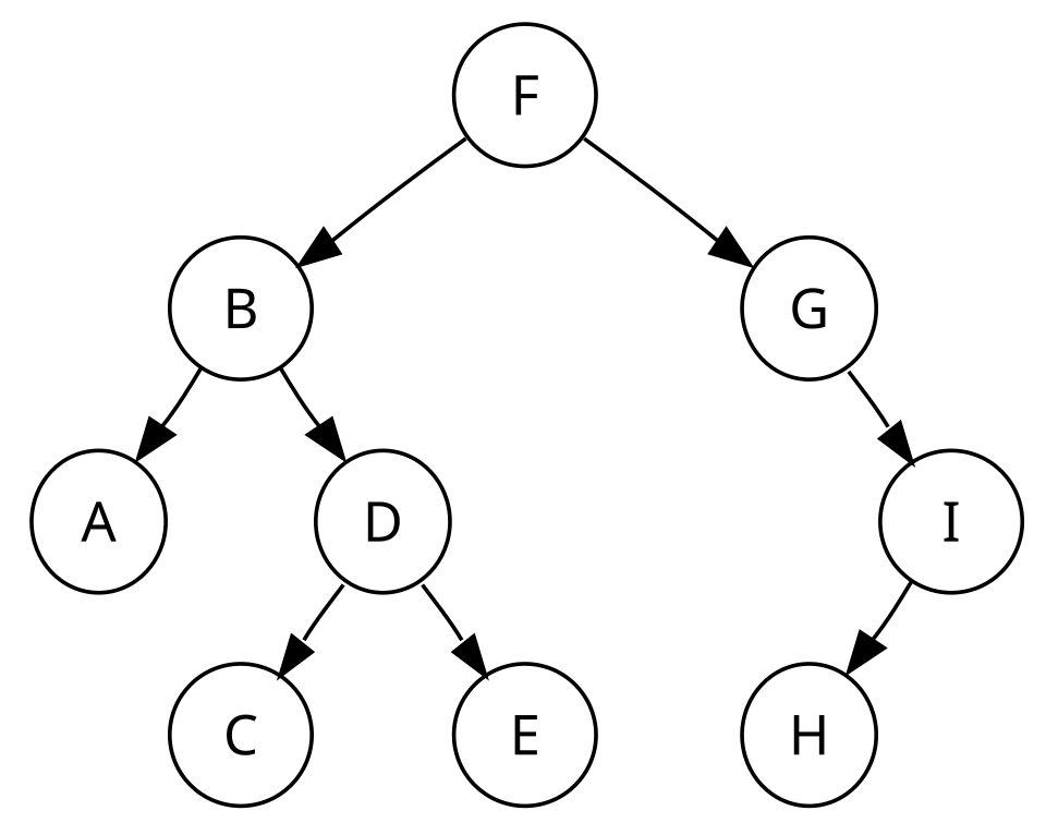Image: A binary tree (sorted, nine nodes), public domain

typedef struct node {
    int          data;
    struct node *left;
    struct node *right;
} node;

A leaf node has both left and right set to NULL.

Special types

Some binary trees have additional structural properties:

Full binary tree

Every node has either 0 or 2 children. There are no “stragglers” — no node with exactly one child. So the tree is completely binary: a node is either a leaf or a fully-branching internal node.

Complete binary tree

Every level is completely filled, except possibly the last — and the last level fills left to right. So if the last level is missing the rightmost node, the tree is still complete. If a node in the middle is missing while ones to its right exist, it’s not complete.

Complete binary trees can be efficiently stored in an array (parent at index $i$ has children at $2 i + 1$ and $2 i + 2$ ). This is exactly how heaps are usually implemented.

Perfect binary tree

Every level is completely filled. A perfect tree of height $h$ has exactly $2^{h + 1} - 1$ nodes. Rare to occur naturally; often used as a theoretical comparison point.

Counting nodes

For a binary tree of height $h$ :

Maximum nodes: $2^{h + 1} - 1$ (perfect tree).
Minimum nodes: $h + 1$ (a left-skewed or right-skewed chain).

So height varies from $⌈ lo g_{2} (n + 1)⌉ - 1$ (best case, balanced) to $n - 1$ (worst case, degenerate chain). This is why balance matters — operations like search are $O (h)$ , so $h = O (lo g n)$ is dramatically better than $h = O (n)$ .

Why binary specifically

Two children is the smallest branching factor that lets you split a problem into halves. Binary search relies on it. Decision-making (yes/no choice) maps onto it. Many algorithms are easier to express recursively when each node has exactly two children to handle — process(node.left) and process(node.right).

When you need higher branching factors (e.g., B-trees with hundreds of children for disk-friendly storage), you use multi-way trees. But for most in-memory data structures, binary is the default.

Visiting all nodes

The four standard ways to traverse a binary tree are pre-order, in-order, post-order, and level-order. Each visits every node exactly once but in a different sequence. See Binary tree traversal for the algorithms and use cases.

Operations

A bare binary tree has no built-in ordering — it’s just a structure. Useful operations require an invariant:

Binary search tree — left subtree < node < right subtree (gives ordered storage with fast search).
Heap (data structure) — parent ≥ children (max-heap) or parent ≤ children (min-heap), gives priority access.
AVL tree / Red-black tree — BSTs with self-balancing rules.

Without one of these invariants, a binary tree is just a record of hierarchical relationships, useful for trees that naturally have hierarchy (parse trees, file systems, expression trees).

Idriss Rami — Notes

Explorer